A theory-heavy intro to machine learning
-1: TLDR
ML syllabi can often feel unmotivated. To fix this, we build up to a notion of inductive bias from scratch and introduce the no-free-lunch theorem.
disclaimer: early draft, may contain errors
0: motivation- a lack of motivation
Virtually every popular machine learning course/text follows some variant of the same syllabus:
- supervised learning
- linear regression, regularization
- classification and logistic regression
- generative algorithms
- kernel methods and SVMs
- deep learning
- MLPs
- backprop
- …
- unsupervised learning
- …
But this syllabus feels extremely unmotivated. It’s the same sort of unsatisfying feeling when learning calculus in a non-rigorous setting for the first time: learning a bunch of random tricks with no global context feelsbadman.
If you crack open the elements of statistical learning for the first time, you’re given a few random examples like digit recognition and then slapped in the face with: “check out this model, it works well”:
\[ \hat{Y} = \hat{\beta}_0 + \sum_{j=1}^p {X}_j \hat{\beta}_j \]
And while I have nothing against linear regression, the obvious question remains:
“why this particular closed form expression?”
In fact, why do we even want any particular closed form expression for a learning problem? Why not just build a universal learner? I.e. a magic linear algebra box that does everything?
By default, this question (which is even more natural in light of the deep-learning meta) will hang over the reader’s head for most of the material covered by such a text. Hence, I’ll start by asking “What is learning, and how should we go about it, a priori of anything?”
(btw if at any point you feel unsatisfied with how i’m explaining things, know that i’m following this text, which has an accompanying series of youtube lectures here)
1: building a formal learning model
Basically we want machines to do our bidding, even in cases where explicitly programming them to do so is impractical. manually if/else-ing your way to self-driving seems pretty rough.
We can put it more formally (Mitchell ’98) (used by Andrew Ng here) as such:
“Well-posed learning Problem: A computer program is said to learn from experience E with respect to some task T and some performance measure P, if its performance on T, as measured by P, improves with experience E”
This is pretty good and i’d advise the reader to try coming up with their own extension of this definition at this point.
Roughly following Shai Shalev-Shwartz, we make a first pass at formalizing this notion:
note: if this feels like it comes out of left-field, seriously try framing it in any other way. It will become clear that you have very few “moves”, and if you do the obvious ones, you end up in basically the exact same place, albeit with probably more esoteric/different notation
We are given:
- some domain \(Z\)
- we don’t just use \(X \times Y\) for observations and labels because unsupervised setups don’t operate on labelled data, and we want generalizable notation. But we can still take \(Z\) to be a cartesian product in the supervised labeled case.
- We assume \(Z\) is a given, but there’s an implicit type/feature representation choice being made for us, i.e. additional bias in the “choice” of feature type. This is beyond the scope of this post, and doesn’t invalidate the subsequent theory, but it’s worth thinking about.
- a training set \(S \subseteq Z\) of examples
- some unknown distribution \(\mathcal{D}\) over \(Z\) which we’d like to model
- and assume the necessary measure-theory considerations hold etc etc
- some set \(\mathcal{H} \subseteq
\mathrm{Fun}(Z, Z)\) of possible models (hypotheses) called a
hypothesis class
- (maybe just every conceivable function from \(Z\) to itself, which is what \(\mathrm{Fun}(Z, Z)\) means)
- example: the set of all linear functions for linear regression
- we take the domain and codomain to be the same, just imagine unseen instances as n-tuples with only n-1 of them filled out, or come up with some other notation. it doesn’t matter
- some “loss function” \(l : Z \times
\mathcal{H} \to \mathbb{R}\) by which we can measure our model
performance.
- technically a functional because we take a model (function) as an input and spit out a real number
- example: zero-one loss, mean squared error, cross-entropy loss, etc…
- we need something to measure how well we do or we literally can’t do anything but guess
- the reals are chosen without loss of generality. pick your favorite ordered field or subset thereof
And we want some algorithm \(A: S \to \mathcal{H}\) that takes our traning set and spits out a good model, i.e.:
\[ A(S) \in \underset{h \in \mathcal{H}}{\mathop{\mathrm{arg\,min}}}\; \mathbb{E}_{z \sim \mathcal{D}}[l(h, z)] \]
which means we want our learning algorithm to give us the lowest expected loss over the true distribution.
Also, as it will be helpful later, let’s define the loss over the true (real world) distribution \({L}_D\) and the loss over our sample \({L}_S\) now:
\[L_\mathcal{D}(h) := \mathbb{E}_{z \sim \mathcal{D}}[l(h, z)]\]
\[{L}_S(h) := \frac{1}{m} \sum_{i=1}^m l(h, {z}_i)\]
for some sample \(S = ({z}_1, \dots, {z}_m) \in Z^m\)
This is still fairly intense notation so let’s run through an example to clarify things:
Let’s say we want to classify papayas as tasty or not tasty, and we represent a papaya by its hardness and color; each of which is a real number scaled to the interval \([0,1]\). Additionally, we have some reason to believe that tasty papayas are ones which are medium-soft and medium-colored, and so for simplicity, that the tasty ones happen to live in some rectangle in \([0,1]^2\).
In this case, our model looks like this:
\(Z := \mathcal{X} \times \mathcal{Y}\) where \(X := [0,1]^2\) and \(Y := \{\pm 1\}\), i.e. our feature space and label space
\(S := \text{ the set of all papayas we've tasted so far }\)
\(\mathcal{H} := \{ \text{ rectangles in } [0,1]^2\}\) viewed as functions which return \(1\) if the papaya lives in the rectangle
${l}_{0-1}(h, (x,y)) := 0 $ if \(h(x) = y\), \(1\) otherwise, where \((x,y) \in \mathcal{X} \times \mathcal{Y} = Z\) i.e. a correctly labelled papaya
note: the subscript 0-1 refers to a binary valued loss, which is typical notation
Now \({L}_D(h)\) just means “what’s the probability \(h\) correctly classifies any real world papaya”
and \({L}_S(h)\) just means “what’s the probability \(h\) correctly classifies a papaya in our sample”.
2: picking an algorithm
How are we supposed to select such a learning algorithm? Note: be careful, when I say “learning algorithm” I do not mean something like stochastic gradient descent. I mean a general process of learning, a framework, a procedure which might give rise to something like SGD. If this is confusing, dw, it will be clear in a moment.
Well, easy! We’ve already seen it: \(\underset{h \in \mathcal{H}}{\mathop{\mathrm{arg\,min}}}\; {L}_\mathcal{D}(h)\)
;;; simply choose the function that minimizes the expected loss over the true distribution

(defun learn (training-data)
  (choose-randomly-from
    (arg-min hypotheses
      (expected-loss-wrt true-distribution loss-function))))
But look carefully; we’ve made a fatal error! Hint: the training-data param is totally unused. What is it? We don’t know the true distribution! Implementing those inner functions would be impossible!
This leaves us with literally one possible move:
;;; simply choose the function that minimizes the expected loss over the *sample*

(defun learn (training-data)
  (choose-randomly-from
    (arg-min hypotheses
      (expected-loss-wrt training-data loss-function))))
note “choose-randomly-from” is glossing over some relatively unimportant detail
Can you spot the difference?
Now we’re minimizing the loss over the sample, not the real distribution:
\[ A(S) \in \underset{h \in \mathcal{H}}{\mathop{\mathrm{arg\,min}}}\; {L}_S(h)\]
We have just discovered a procedure called Expected Risk Minimization (ERM), which forms the basis for virtually every machine learning algorithm out there. We call it this because \({L}_S\) is usually referred to as the sample loss or training error or training risk or empirical risk (depending on who you ask).
We still haven’t answered our original question about why we bother with closed-form solutions and very particular models, but we’re getting there.
The next reasonable question is whether or not we expect to get anything out of this learning paradigm at all. I.e., what guarantees will doing ERM give us? Is it really reasonable to expect that fitting our model to the sample will help us generalize to the real world?
Well, currently, no. Recall the papaya example, where a labelled papaya is of the form \((x,y)\), and consider the following hypothesis \(h_m \in \mathcal{H}\) (subscript m for memorize):
\[ h_m(x) = \begin{cases} y_i & \text{if } \exists (x_i, y_i) \in S \text{ such that } x = x_i, \\ 1 & \text{otherwise} \end{cases} \]
in other words: to predict a new papaya \(x\), check if there’s one in the training set which looks exactly like \(x\), and if so, return its label. Otherwise, guess a hardcoded label.
Clearly this will correctly predict every single training example, so \(L_S(h_m) = 0\), and so \(ERM_{\mathcal{H}}\) can trivially return this function, which will probably perform very poorly in the real world. If the real distribution is 50/50, and there are many many more papayas than just the ones we’ve seen, this hypothesis will get 100% training accuracy and roughly 50% test-time accuracy (no better than chance). If the real distribution is 90/10 and our hardcoded label points at the latter, we’d get 10% test-time accuracy. Not good!
3: moving the goalposts: PAC
So it looks like we only have one “move”: find functions that minimize sample loss; but if we use this tool naively, and just search over all possible functions, we’re going to “overfit” the data and fail miserably.
Maybe there’s a way to fix this obvious problem, but first we should specify in greater detail what it is that we want out of our learning framework, so we can come back and revise our earlier definition with this goal in mind.
note that we still have ways to revise ERM; namely the set \(\mathcal{H}\) which we minimize the loss over…
Colloquially, we don’t want overfitting, i.e. doing well on the training set but badly in the real world.
Let’s require that our learning algorithm \(A\) over a domain \(Z\) return a hypothesis \(h\) with the property that, for any distribution \(\mathcal{D}\) over \(Z\):
\[ L_D(h) = 0\]
Well, that would avoid the previous problem, but it’s not clear that such an algorithm would even exist; due to noise, outliers, etc…, it’s pretty unlikely that any hypothesis will have exactly zero loss in the real world. OK, let’s revise:
We’ll now only require that:
\[L_D(h) \leq \epsilon\]
for some \(\epsilon \in (0,1)\), i.e. we have some accuracy tolerance \(\epsilon\)
But there’s another problem: how do we select a reasonable \(\epsilon\)? We’d have to know exactly how much error to expect from the true distribution… OK, another revision is needed:
\[L_D(h) \leq \min_{h' \in \mathcal{H}} L_D(h') + \epsilon\]
Now we require only that \(A\) returns an \(h\) which is within \(\epsilon\) of the best we could ever hope to do on the given problem we’re trying to solve. So if we’re predicting coin tosses, this would be \(1/2 + \epsilon\).
…But if we are predicting coin tosses, and our sample \(S\) only has heads, just by bad luck, we’re never going to succeed. In other words, we need to account for the chance that we get a nonrepresentative sample:
\[\exists m \in \mathbb{N} : |S| \geq m \implies \mathbb{P}_{S \sim \mathcal{D}^m} [L_D(h_S) \geq \min_{h \in \mathcal{H}} L_D(h) + \epsilon] \leq \delta\]
i.e., there is some number of samples \(m\) we can take to ensure that the chance the algorithm returns a shitty hypothesis is less than some “confidence parameter” \(\delta\). In this case “shitty hypothesis” means \(L_D(h) \geq \min_{h' \in \mathcal{H}} L_D(h') + \epsilon\), i.e. we are more than epsilon worse than what we are shooting for i.e. just reversing the equality in the previous constraint. (you could equivalently say we want greater than \((1-\delta)\) chance of satisfying the previous \(\leq\)-defined constraint)
OK, I swear we’re done now! You can now view \(m\) as a function of \((\epsilon, \delta)\) that returns the minimum number of samples needed to ensure that our algorithm is probably (with confidence \(1-\delta\)) approximately (within \(\epsilon\) tolerance) correct.
All together, we have just worked our way up from first principles to the following definition from Shwartz’ understanding machine learning, from theory to algorithms:
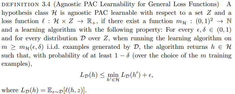
4: hitting the goalposts- finite hypothesis classes
Now that we have a clear criterion for acceptable learning algorithms (PAC learnability), we should alter our original ERM setup and check if we satisfy this criterion.
Note that since PAC learnability is a property of the chosen hypothesis class we’re trying to learn, we will only have to adjust the hypothesis class to which we apply the ERM algorithm.
The clear adjustment to make is a restriction of \(\mathcal{H}\) to the finite case, so that it does not include trivially bad functions like “memorize the sample set”. Intuitively, the bad “memorize” hypothesis we’re trying to avoid belongs to a family of functions which would require an infinitely long lookup table, and is thus excluded in the restriction to the finite case.
The question now is “does our first attempt, i.e. restricting \(\mathcal{H}\) to the finite case, actually give us that \(\mathcal{H}\)” is PAC-learnable? It turns out the answer is yes.
I’ll skip the proof, which you can read if you’re interested (roughly page 55 in the linked text), but the main idea is that by requiring \(|\mathcal{H}| \leq \infty\), we can use the union bound (\(P(A \cup B) \leq P(A) + P(B)\)) and Hoeffding’s inequality to get the following result:
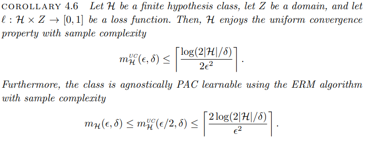
Here, \(m_{\mathcal{H}}\) is the minimum number of samples required to garuntee that our learning algorithm will be probably approximately correct.
Note that if we tighten our error tolerance (decrease \(\epsilon\)), tighten our confidence bound (decrease \(\delta\)), or increase the scope of our model (increase \(\mathcal{H}\)) we will need more samples to get the same garuntee.
In other words: a broad hypothesis class will require more samples than a narrow one to acheive good performance
5: quick recap
So far, this may feel very detached from reality, and it feels like all we’ve done is manipulate definitions, but we’ve actually uncovered two very deep truths from scratch:
- our standard learning paradigm will be minimizing loss on the training set
- a good way to avoid bad outcomes is to restrict the set of admissable models
Next, we will consider point 2 in more depth.
6: the bias-variance tradeoff
We have observed that restricting the size of \(\mathcal{H}\) can help in avoiding overfitting. The natural question remains: what are the drawbacks?
Well, our PAC definition gives us garuntees about ERM performance only with respect to the best possible model in our given hypothesis class: This is what is meant by the min of \(h'\) in the PAC statement \(L_\mathcal{D}(h) \leq \min_{h' \in \mathcal{H}} L_\mathcal{D}(h') + \epsilon\)
So we can think about the size of \(\mathcal{H}\) as follows. If we’re approaching a learning problem and have a fixed number of samples:
Large \(\mathcal{H} \implies\)
- increased risk of overfitting (recall the sample complexity bound obtained earlier)
- increased chance that some \(h \in \mathcal{H}\) will be able to model the true distribution
equivalently, a small \(\mathcal{H} \implies\)
- lower chance of overfitting
- higher chance that no model in \(\mathcal{H}\) will be powerful enough to model the true distribution
To line our observations up with standard terminology, we say:
Restricting \(\mathcal{H}\) (trading away model complexity) amounts to introducing inductive bias which:
- may increase the approximation error
- aka increases the loss of the best possible \(h \in \mathcal{H}\)
- our restriction may be so severe we can’t capture the essence of the true distribution
- may decrease the estimation error
- aka the difference between the loss on the sample vs the loss on the true distribution
- our restriction saves us from effectively memorizing the sample and losing predictive power
We call it inductive bias because it reflects the use of prior knowledge about the distribution to narrow our set of possible hypotheses and thus avoid higher sample complexity and overfitting risk, at the cost of robustness.
7: the no-free-lunch theorem
At this point, the only remaining question is “why not build a universal learner?”
We’ve shown that, in practice, introducing inductive bias can be a good strategy to approach learning problems, as it can alleviate the natural risk of overfitting to data, and reduce the amount of data we need to see.
I like to think of it as: modeling a low-entropy distribution with an overpowered model will naturally introduce noise, and modeling a high-entropy distribution with an underpowered model will naturally underperform.
However, we haven’t ruled out the possibility of a learner that solves every problem. If such a thing were possible, we should probably spend all our time on that, so it’s worth ruling it out.
There’s an often-cited theorem from Statistical Learning Theory that addresses this. From the text:
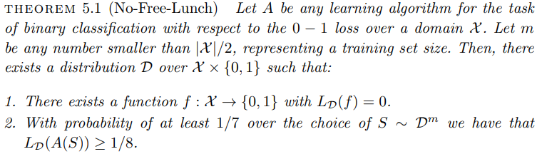
This is pretty opaque, so let’s consider the colloquial phrasing and go from there:
“This theorem states that for every learner, there exists a task on which it fails”
Seems pretty reasonable, but I think we can get a better intuition by rephrasing it, taking note of the fixed sample size in the definition. I’ll say instead:
“For any fixed, reasonable sample size from a domain \(\mathcal{X}\), no learner can guarantee high accuracy and confidence for all possible distributions \(\mathcal{D}\) over \(\mathcal{X}\)”
This seems more immediately believable to me, but we can do better by supposing it’s false and going by contradiction. Then we’d have that:
“For a fixed, reasonable sample size over a domain \(\mathcal{X}\), there exists a learner which gives arbitrarily good \((\epsilon, \delta)\) performance on every distribution \(\mathcal{D}\) over \(\mathcal{X}\).
This seems highly implausible, reinforcing the idea that no single learner can be optimal for all possible distributions. To understand this better, consider an analogous (though very loosely phrased) statement: ‘The uncertainty in any distribution \(\mathcal{D}\) can be fully captured by a smaller sample \(S\),’ or equivalently, ‘we can losslessly compress any data distribution.’ Clearly, this is false, as we cannot capture all the variability of any distribution in a finite sample without some loss of information.
I’m not going to go through the formal proof here, because it’s notationally cumbersome, but the core idea is pretty straightforward and you can see a sketch of it in this video.
That said, the intuitive proof-by-contradiction feels pretty solid, at least to me.
The elephant in the room is bascially the objection “wait, I feel like gpt4 is a pretty universal learner; it knows natural language which can express pretty much anything…”.
The counterpoint is that GPT-4 and similar models incorporate significant inductive biases in their architectures, (e.g. assumptions about token dependencies) which necessarily limit their universality across different types of data distributions. Just because the model has good real-life generalization capabilities does not mean it can accurately model literally every pathological distribution over token sequences.
8: conclusion:
If all of this theory feels useless, like we basically just played with definitions and notations, that’s OK. When we started, it wasn’t clear that we wanted to choose an inductive bias at all, or that minimizing the sample loss was the way to go, but hopefully now these feel like the natural and obvious things to do.
For advanced practitioners, this might feel silly, but I remember taking a grad-level machine learning course as an undergrad and was very confused at the start why we took such things for granted. Maybe others just see these as obvious, but I certainly had to spend a few days thinking about it. This writeup was done to clarify my own understanding of some of the basics of statistical learning.