optimization techniques
jan 19, 2026
recap
We’re working our way up to modern transformer-based language models, and we’ve covered the basics of how to approach learning in general.
The basic regime we’re following is:
- choose a sample \(S\) (training set) from the distribution we want to model
- choose a loss function \(\ell\) that measures prediction error
- choose a ‘hypothesis class’ (~model architecture) \(H\)
Then, we find a function \(h \in H\) which minimizes the empirical risk over \(S\).
optimization
Now we’re asking an optimization question. We’re just minimizing some objective function. And at this point, we don’t have any constraints on what the objective or loss functions look like.
This means we probably want to look for techniques which place minimal constraints on our objective function.
For instance, there are a bunch of EM-based procedures and bayesian frameworks for learning. With these, the idea is to pick some nice distribution as the hypothesis class, and use variations on the Expectation-Maximization algorithm to estimate its parameters. The problem there is that integrating your priors needs to be analytically tractable.
Even if we think of more classical optimization methods like ‘set derivative equal to zero and solve’, again we’re faced with analytical intractability. Other popular optimization algorithms include things like linear programming. But then the objective function needs to be linear and convex. And those are pretty stringent requirements that would make life extremely difficult.
Fortunately, there is an iterative optimization algorithm that only imposes one requirement: differentiability in the objective and loss functions.
gradient descent
First, it’s worth mentioning that the differentiability requirement does mean that we’re making another assumption on the functional form of our model.
Namely, that our model \(h_\theta : \mathbb{R}^n \to \mathbb{R}^m\) is differentiable with respect to its parameters \(\theta\). Before, we had no such restriction. This means that we’re going to have to convert our model inputs to real-valued vectors, and our loss function is also going to have to be differentiable.
Let’s say our model is \(h_\theta\) and our loss function for a single example is \(\ell(h_\theta(x), y)\) where \(y\) is the true label.
According to the ERM procedure, we need to minimize our average sample loss:
\[ L_S(\theta) := \frac{1}{N}\sum_{i=1}^{N} \ell(h_\theta(x_i), y_i) \;\; \text{for} \;\; (x_i, y_i) \in S \]
Gradient descent does this by setting, for some small ‘step size’ \(\eta\):
\[ \begin{align} \theta_0 &:= \text{random} \\ \theta_{t+1} &:= \theta_t - \eta \nabla_\theta L_S(\theta_t) \\ &= \theta_t - \frac{\eta}{N}\sum_{i=1}^{N} \nabla_\theta \ell(h_\theta(x_i), y_i) \bigg|_{\theta=\theta_t} \end{align} \]
In other words, we literally just follow the gradient around the loss landscape for some arbitrary number of iterations until we’re happy.
In python, a barebones implementation for a random function on \(\mathbb{R}^2\) looks like:
def gd(grad_fn, start, n_steps, stepsize):
    x, y = start
    for _ in range(n_steps):
        gx, gy = grad_fn(x,y)
        x -= stepsize * gx
        y -= stepsize * gy
    return x,y
worked example
Ok let’s pick a trivial example.
Consider the function \(f(x, y) = 1 +
\sin(x) + \cos(y) + \frac{1}{10}(y + y^2 + x^2)\). 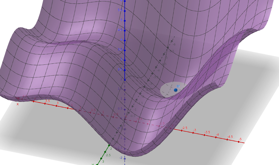
As you can see, we have a nice little example with some local minima to play with.
We can manually derive the gradient: \[ \nabla f(x, y) = \begin{pmatrix} \cos(x) + \frac{1}{5}x \\ -\sin(y) + \frac{1}{10} + \frac{1}{5}y \end{pmatrix} \]
# arbitrary function with some local minima
def f(x, y):
    return 1 + sin(x) + cos(y) + (1/10)* (y + y**2 +x^2)

# hand-derived gradient
def grad_f(x,y):
    grad_x = cos(x) + (1/5) * x
    grad_y = -sin(y) + 1/10 + (1/5) * y
    return grad_x, grad_y

# hand-derived analytical solution
def f_argmin():
    return -1.32, -2.68
By manual ‘set-derivative-equal-to-zero’ method we know the solution should be around \((-1.32, -2.68)\)
Does gradient descent work? …
(ml2) ❄️ ~/projects/ml2/ml2 λ python main.py
gd(0, 0) => (-1.31,-2.69)(True) w/ stepsize=0.01 in 1000 steps
gd(4, 2) => (3.84,2.50)(False) w/ stepsize=0.01 in 1000 steps
Sometimes! But we get trapped in local minima.
You can imagine the procedure as hill descending. Like a ball. But our ball has no momentum.
What if we add some? By that, I mean literally add a velocity term \(\mu\), where we just carry over some of the previous gradient information to the present iteration:
\[ \begin{align} \theta_0 &:= \text{random} \\ v_0 &:= 0 \\ v_{t+1} &:= \mu v_t + \eta \nabla_\theta L_S \\ \theta_{t+1} &:= \theta_t - v_{t+1} \end{align} \]
In code:
# gd with momentum (sutskever version)
def momentum(grad_fn, start, n_steps, stepsize, mu):
    x, y = start
    vx, vy = 0,0
    for _ in range(n_steps):
        g = grad_fn(x,y)
        vx = mu * vx + stepsize * g[0]
        vy = mu * vy + stepsize * g[1]
        x -= vx
        y -= vy

    return x, y
Does this version work?
(ml2) ❄️ ~/projects/ml2/ml2 λ python main.py
momentum(0, 0) => (-1.30,-2.68)(True) w/ stepsize=0.01 in 1000 steps
momentum(10, 10) => (-1.30,-2.69)(True) w/ stepsize=0.01 in 1000 steps
Yes …
We can also see the convergence plots. I.e., how far away from the optimum are we at each step of gradient descent? For standard GD and the momentum version:
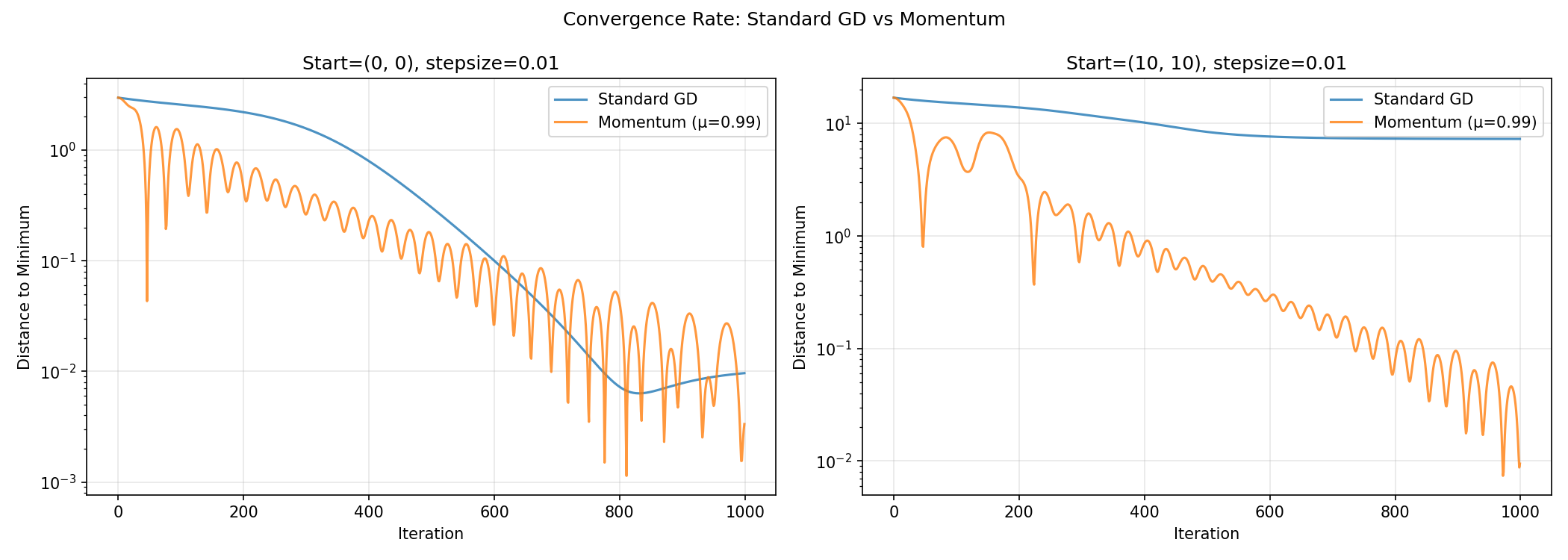
Its funny the extent to which the convergence plot follows physical intuition. As an aside, you can prove properties about convergence (usually limited to L-smooth convex functions) using an ODE dual formulation with physics-like position and velocity components. That’s for a followup (if ever) though.
Also, I lied earlier.
(ml2) ❄️ ~/projects/ml2/ml2 λ python main.py
gd(0, 0) => (-1.31,-2.69)(True) w/ stepsize=0.01 in 1000 steps
gd(4, 2) => (3.84,2.50)(False) w/ stepsize=0.01 in 1000 steps
momentum(0, 0) => (-1.30,-2.68)(True) w/ stepsize=0.01 in 1000 steps
momentum(4, 2) => (3.84,2.50)(False) w/ stepsize=0.01 in 1000 steps
Because the function I chose is actually pretty pathological and nasty, we can still pick starting points where momentum sgd fails to converge to the global optimum.
So. Yeah it’s not foolproof.
gradient computation, sgd
In our toy example, we literally just optimized an arbitrary function.
In reality, in a real optimize-the-model scenario, we are optimizing parameters, and we’re computing the average gradient- i.e. not just at one point, but at all the points in the sample set.
The problem with this is that it becomes computationally intractable at large sample sizes.
The solution is to just compute the average over a small batch of samples. This is called stochastic gradient descent and is the real one people use in practice.
better versions
One improvement is called the nesterov method where instead of computing the gradient at the current weights \(\theta_t\) you compute the next gradient at a lookahead point \(\theta_t - \mu v_t\).
This is nice because if your loss landscape is brutal (ratio of smallest to largest eigenvalue of the hessian is really high), the lookahead version cancels some of the oscillation that would happen.
Other popular variants like adamW adjust hyperparameters in smarter ways than just “keep the learning rate the same the whole time”.
I might do a followup post on adamW but for now we have a good enough tool.