model architecture

Jan 22 2026

Last time we introduced gradient descent. Now we ought to choose a model architecture.

Of course, it’d be absurd to try and pick a full model architecture at this point. We don’t have any empirical data. We have a few a priori notions about some broad theoretical ideas. That’s it.

However, if you recall from last time, our hand is at this point already somewhat forced:

we’re making another assumption on the functional form of our model. Namely, that our model \(h_\theta : \mathbb{R}^n \to \mathbb{R}^m\) is differentiable with respect to its parameters \(\theta\).

Also it’s worth typechecking the model input/output quickly. Recall we’re trying to model language so we have something like:

\[ \text{text} \xrightarrow[\text{?}]{} \begin{pmatrix} x_1 \\ \vdots \\ x_n \end{pmatrix} \xrightarrow[f_\theta]{} \begin{pmatrix} y_1 \\ \vdots \\ y_m \end{pmatrix} \xrightarrow[\ell]{} \mathbb{R} \]

So now the question is… which functional form should \(f_\theta\) take?

Let’s think about our criteria, in order of most to least important:

differentiable
expressive; can approximate arbitrary (reasonably nice) functions
efficiently computable, numerically stable
works well with vectorized input

any guesses?

the original universal approximation theorem

At this point, at least for me, the following theorem jumps to mind:

Stone-Weierstrass Approximation Theorem: Suppose \(f\) is a continuous real-valued function defined on the real interval \([a, b]\). For every \(\epsilon > 0\), there exists a polynomial \(p\) such that for all \(x\) in \([a, b]\), we have \(|f(x) - p(x)| < \epsilon\)

In other words, polynomials fit the bill pretty well. So that’s the solution then, right? just stack polynomials?

But then like… how would we do that? Something like:

\[ f_i(x_i) = a_0 + a_1 x_i + a_2 x_i^2 + \dots + a_n x_i^n \]

This looks reasonable but also it doesn’t really fit our criteria:

✅ polynomials are definitely differentiable
✅ polynomials can approximate most functions we care about
❌ high degree polynomials are extremely numerically unstable, and no hardware-level support
❌ component-wise evaluation is ugly, we lose a lot of information

So we’re close, but not quite.

What about if we formulated the polynomial with cross terms:

\[ f(x_1, \dots, x_n) = \sum_{k_1 + \dots + k_n \leq d} a_{k_1 \dots k_n} x_1^{k_1} \cdots x_n^{k_n} \]

Well ok so if we did this, we don’t ‘lose information’ but now we have a parameter explosion; estimating parameters there is \(O(n^d)\)… grossly inefficient. So that’s really no help. We’re still only hitting half our criteria.

mlp universal approximation theorem

Fortunately, it turns out there’s another family of functions that does satisfy these criteria: chained compositions of affine linear transformations and nonlinear ‘activation’ functions:

\[ \sigma(W_2 \cdot \sigma(W_1 x + b_1) + b_2) \]

where \(W \in \mathbb{R}^{m \times n}\), \(b \in \mathbb{R}^m\), and \(\sigma\) is a non-polynomial continuous function (e.g. sigmoid, ReLU).

You’ve probably heard of these. We call them MLPs (multilayer perceptrons). You’ve probably seen the classic image (which personally I find misleading and ugly compared to the symbolic form but whatever):

And, fortunately, it turns out we have theorems proving that functions of this form are able to approximate reasonably ‘nice’ functions.

There are various forms of the theorem for various levels of ‘nice’ function (continuous, lebesgue integrable, continuously differentiable, etc…) and different nonlinear activations \(\sigma\).

I’m not going to prove the theorem here, but the basic idea is this (wlog, for dim=1):

use weighted sums of expressions of the form \(\sigma(ax +b)\) to produce stairsteps
combine the stairsteps to fit your function
increase the number of stairsteps arbitrarily a la riemann integration

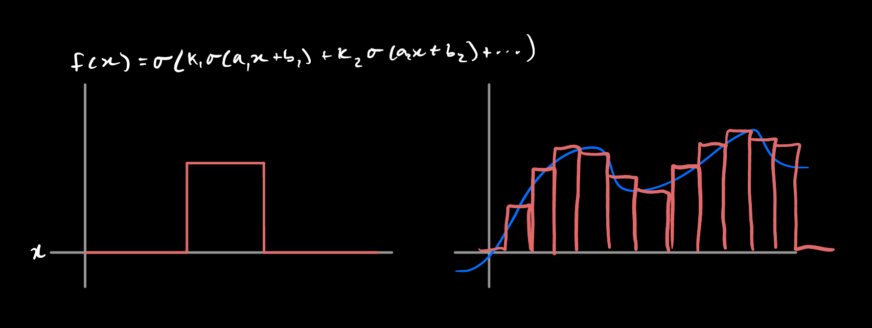
This site has a pretty solid explainer if you want more depth, but they use a nonlinearity of the form \(\sigma = (1+e^{-x})^{-1}\), i.e. the classic sigmoid.

But we’re building up from scratch and it’s not clear why we’d choose that nonlinearity.

Fortunately some of those approximation theorems also work for the dumbest possible nonlinearity, the ReLu (rectified linear unit) function:

\[ \mathrm{ReLu}(x) := \mathrm{max}(0, x) \]

And instead of stairsteps, the visual proof intuition is more like jagged peaks, since the ReLu function technically isn’t sigmoidal (it goes off to \(+\infty\)).

You can spend 15 minutes in desmos to grok the intuition if you aren’t sold.

recap

Let’s make sure our new candidate functional form actually checks our boxes:

✅ affine linear transformations and relu are differentiable (x=0 is measure 0 so just be a good little engineer and pretend that max function is differentiable at zero with derivative 1 or 0 depending on your preference)
✅ we have universal approximation theorems saying we can approximate lots of functions
✅ the computation here boils down to matmul, and hardware acceleration for this is a trillion dollar industry
✅ this trivially plays nice with vector inputs, with managable layer-wise computational complexity \(O(m \times n)\) for \(W \in \mathbb{R}^{m \times n}\)

Great!

I’ve gone kind of fast so here’s the new picture:

One Layer: \[ \text{text} \Rightarrow \begin{bmatrix} x_1 \\ x_2 \\ \vdots \\ x_n \end{bmatrix} \xrightarrow{L_1} \begin{bmatrix} \sigma(w_{11}x_1 + w_{12}x_2 + \cdots + w_{1n}x_n + b_1) \\ \sigma(w_{21}x_1 + w_{22}x_2 + \cdots + w_{2n}x_n + b_2) \\ \vdots \\ \sigma(w_{m1}x_1 + w_{m2}x_2 + \cdots + w_{mn}x_n + b_m) \end{bmatrix} = \sigma(Wx + b) \]

N layers:

\[ \text{text} \Rightarrow \mathbb{R}^n \xrightarrow{L_1} \mathbb{R}^m \rightarrow \cdots \rightarrow \mathbb{R}^k \xrightarrow{L} \mathbb{R} \]

So at this point, here’s what we have left to do before we can start doing language modeling:

figure out what loss function to use
get some data to test on
figure out how to encode the data into euclidean space
decide hyperparameters; how wide should the network be? sgd learning rate? etc…

Next time we’ll look at loss functions!