ml blogpost series overview
jan 19 2026
This is a short series of blogposts intended to work up to modern language and image models from ‘scratch’.
I’m mostly writing this for myself- I tend to learn best when i’m forced to explain things. But others may find it useful.
chapters
- ml1- intro theory
- theoretical learning background. skippable if you understand the motivation behind ‘optimize a loss function over a training set’ or just buy that that’s a sensible thing to do.
- ml2- optimization
- basic optimization stuff, gradient descent
- ml3- architecture
- universal approximation, why MLPs are a reasonable functional form
- ml4- loss functions
- softmax, cross-entropy loss, perplexity
A theory-heavy intro to machine learning
jan 19 2026
-1: TLDR
ML syllabi can often feel unmotivated. To fix this, we build up to a notion of inductive bias from scratch and introduce the no-free-lunch theorem.
disclaimer: early draft, may contain errors
0: motivation- a lack of motivation
Virtually every popular machine learning course/text follows some variant of the same syllabus:
- supervised learning
- linear regression, regularization
- classification and logistic regression
- generative algorithms
- kernel methods and SVMs
- deep learning
- MLPs
- backprop
- …
- unsupervised learning
- …
But this syllabus feels extremely unmotivated. It’s the same sort of unsatisfying feeling when learning calculus in a non-rigorous setting for the first time: learning a bunch of random tricks with no global context feelsbadman.
If you crack open the elements of statistical learning for the first time, you’re given a few random examples like digit recognition and then slapped in the face with: “check out this model, it works well”:
\[ \hat{Y} = \hat{\beta}_0 + \sum_{j=1}^p {X}_j \hat{\beta}_j \]
And while I have nothing against linear regression, the obvious question remains:
“why this particular closed form expression?”
In fact, why do we even want any particular closed form expression for a learning problem? Why not just build a universal learner? I.e. a magic linear algebra box that does everything?
By default, this question (which is even more natural in light of the deep-learning meta) will hang over the reader’s head for most of the material covered by such a text. Hence, I’ll start by asking “What is learning, and how should we go about it, a priori of anything?”
(btw if at any point you feel unsatisfied with how i’m explaining things, know that i’m following this text, which has an accompanying series of youtube lectures here)
1: building a formal learning model
Basically we want machines to do our bidding, even in cases where explicitly programming them to do so is impractical. manually if/else-ing your way to self-driving seems pretty rough.
We can put it more formally (Mitchell ’98) (used by Andrew Ng here) as such:
“Well-posed learning Problem: A computer program is said to learn from experience E with respect to some task T and some performance measure P, if its performance on T, as measured by P, improves with experience E”
This is pretty good and i’d advise the reader to try coming up with their own extension of this definition at this point.
Roughly following Shai Shalev-Shwartz, we make a first pass at formalizing this notion:
note: if this feels like it comes out of left-field, seriously try framing it in any other way. It will become clear that you have very few “moves”, and if you do the obvious ones, you end up in basically the exact same place, albeit with probably more esoteric/different notation
We are given:
- some domain \(Z\)
- we don’t just use \(X \times Y\) for observations and labels because unsupervised setups don’t operate on labelled data, and we want generalizable notation. But we can still take \(Z\) to be a cartesian product in the supervised labeled case.
- We assume \(Z\) is a given, but there’s an implicit type/feature representation choice being made for us, i.e. additional bias in the “choice” of feature type. This is beyond the scope of this post, and doesn’t invalidate the subsequent theory, but it’s worth thinking about.
- a training set \(S \subseteq Z\) of examples
- some unknown distribution \(\mathcal{D}\) over \(Z\) which we’d like to model
- and assume the necessary measure-theory considerations hold etc etc
- some set \(\mathcal{H} \subseteq
\mathrm{Fun}(Z, Z)\) of possible models (hypotheses) called a
hypothesis class
- (maybe just every conceivable function from \(Z\) to itself, which is what \(\mathrm{Fun}(Z, Z)\) means)
- example: the set of all linear functions for linear regression
- we take the domain and codomain to be the same, just imagine unseen instances as n-tuples with only n-1 of them filled out, or come up with some other notation. it doesn’t matter
- some “loss function” \(l : Z \times
\mathcal{H} \to \mathbb{R}\) by which we can measure our model
performance.
- technically a functional because we take a model (function) as an input and spit out a real number
- example: zero-one loss, mean squared error, cross-entropy loss, etc…
- we need something to measure how well we do or we literally can’t do anything but guess
- the reals are chosen without loss of generality. pick your favorite ordered field or subset thereof
And we want some algorithm \(A: S \to \mathcal{H}\) that takes our traning set and spits out a good model, i.e.:
\[ A(S) \in \underset{h \in \mathcal{H}}{\mathop{\mathrm{arg\,min}}}\; \mathbb{E}_{z \sim \mathcal{D}}[l(h, z)] \]
which means we want our learning algorithm to give us the lowest expected loss over the true distribution.
Also, as it will be helpful later, let’s define the loss over the true (real world) distribution \({L}_D\) and the loss over our sample \({L}_S\) now:
\[L_\mathcal{D}(h) := \mathbb{E}_{z \sim \mathcal{D}}[l(h, z)]\]
\[{L}_S(h) := \frac{1}{m} \sum_{i=1}^m l(h, {z}_i)\]
for some sample \(S = ({z}_1, \dots, {z}_m) \in Z^m\)
This is still fairly intense notation so let’s run through an example to clarify things:
Let’s say we want to classify papayas as tasty or not tasty, and we represent a papaya by its hardness and color; each of which is a real number scaled to the interval \([0,1]\). Additionally, we have some reason to believe that tasty papayas are ones which are medium-soft and medium-colored, and so for simplicity, that the tasty ones happen to live in some rectangle in \([0,1]^2\).
In this case, our model looks like this:
\(Z := \mathcal{X} \times \mathcal{Y}\) where \(X := [0,1]^2\) and \(Y := \{\pm 1\}\), i.e. our feature space and label space
\(S := \text{ the set of all papayas we've tasted so far }\)
\(\mathcal{H} := \{ \text{ rectangles in } [0,1]^2\}\) viewed as functions which return \(1\) if the papaya lives in the rectangle
${l}_{0-1}(h, (x,y)) := 0 $ if \(h(x) = y\), \(1\) otherwise, where \((x,y) \in \mathcal{X} \times \mathcal{Y} = Z\) i.e. a correctly labelled papaya
note: the subscript 0-1 refers to a binary valued loss, which is typical notation
Now \({L}_D(h)\) just means “what’s the probability \(h\) correctly classifies any real world papaya”
and \({L}_S(h)\) just means “what’s the probability \(h\) correctly classifies a papaya in our sample”.
2: picking an algorithm
How are we supposed to select such a learning algorithm? Note: be careful, when I say “learning algorithm” I do not mean something like stochastic gradient descent. I mean a general process of learning, a framework, a procedure which might give rise to something like SGD. If this is confusing, dw, it will be clear in a moment.
Well, easy! We’ve already seen it: \(\underset{h \in \mathcal{H}}{\mathop{\mathrm{arg\,min}}}\; {L}_\mathcal{D}(h)\)
;;; simply choose the function that minimizes the expected loss over the true distribution

(defun learn (training-data)
  (choose-randomly-from
    (arg-min hypotheses
      (expected-loss-wrt true-distribution loss-function))))
But look carefully; we’ve made a fatal error! Hint: the training-data param is totally unused. What is it? We don’t know the true distribution! Implementing those inner functions would be impossible!
This leaves us with literally one possible move:
;;; simply choose the function that minimizes the expected loss over the *sample*

(defun learn (training-data)
  (choose-randomly-from
    (arg-min hypotheses
      (expected-loss-wrt training-data loss-function))))
note “choose-randomly-from” is glossing over some relatively unimportant detail
Can you spot the difference?
Now we’re minimizing the loss over the sample, not the real distribution:
\[ A(S) \in \underset{h \in \mathcal{H}}{\mathop{\mathrm{arg\,min}}}\; {L}_S(h)\]
We have just discovered a procedure called Expected Risk Minimization (ERM), which forms the basis for virtually every machine learning algorithm out there. We call it this because \({L}_S\) is usually referred to as the sample loss or training error or training risk or empirical risk (depending on who you ask).
We still haven’t answered our original question about why we bother with closed-form solutions and very particular models, but we’re getting there.
The next reasonable question is whether or not we expect to get anything out of this learning paradigm at all. I.e., what guarantees will doing ERM give us? Is it really reasonable to expect that fitting our model to the sample will help us generalize to the real world?
Well, currently, no. Recall the papaya example, where a labelled papaya is of the form \((x,y)\), and consider the following hypothesis \(h_m \in \mathcal{H}\) (subscript m for memorize):
\[ h_m(x) = \begin{cases} y_i & \text{if } \exists (x_i, y_i) \in S \text{ such that } x = x_i, \\ 1 & \text{otherwise} \end{cases} \]
in other words: to predict a new papaya \(x\), check if there’s one in the training set which looks exactly like \(x\), and if so, return its label. Otherwise, guess a hardcoded label.
Clearly this will correctly predict every single training example, so \(L_S(h_m) = 0\), and so \(ERM_{\mathcal{H}}\) can trivially return this function, which will probably perform very poorly in the real world. If the real distribution is 50/50, and there are many many more papayas than just the ones we’ve seen, this hypothesis will get 100% training accuracy and roughly 50% test-time accuracy (no better than chance). If the real distribution is 90/10 and our hardcoded label points at the latter, we’d get 10% test-time accuracy. Not good!
3: moving the goalposts: PAC
So it looks like we only have one “move”: find functions that minimize sample loss; but if we use this tool naively, and just search over all possible functions, we’re going to “overfit” the data and fail miserably.
Maybe there’s a way to fix this obvious problem, but first we should specify in greater detail what it is that we want out of our learning framework, so we can come back and revise our earlier definition with this goal in mind.
note that we still have ways to revise ERM; namely the set \(\mathcal{H}\) which we minimize the loss over…
Colloquially, we don’t want overfitting, i.e. doing well on the training set but badly in the real world.
Let’s require that our learning algorithm \(A\) over a domain \(Z\) return a hypothesis \(h\) with the property that, for any distribution \(\mathcal{D}\) over \(Z\):
\[ L_D(h) = 0\]
Well, that would avoid the previous problem, but it’s not clear that such an algorithm would even exist; due to noise, outliers, etc…, it’s pretty unlikely that any hypothesis will have exactly zero loss in the real world. OK, let’s revise:
We’ll now only require that:
\[L_D(h) \leq \epsilon\]
for some \(\epsilon \in (0,1)\), i.e. we have some accuracy tolerance \(\epsilon\)
But there’s another problem: how do we select a reasonable \(\epsilon\)? We’d have to know exactly how much error to expect from the true distribution… OK, another revision is needed:
\[L_D(h) \leq \min_{h' \in \mathcal{H}} L_D(h') + \epsilon\]
Now we require only that \(A\) returns an \(h\) which is within \(\epsilon\) of the best we could ever hope to do on the given problem we’re trying to solve. So if we’re predicting coin tosses, this would be \(1/2 + \epsilon\).
…But if we are predicting coin tosses, and our sample \(S\) only has heads, just by bad luck, we’re never going to succeed. In other words, we need to account for the chance that we get a nonrepresentative sample:
\[\exists m \in \mathbb{N} : |S| \geq m \implies \mathbb{P}_{S \sim \mathcal{D}^m} [L_D(h_S) \geq \min_{h \in \mathcal{H}} L_D(h) + \epsilon] \leq \delta\]
i.e., there is some number of samples \(m\) we can take to ensure that the chance the algorithm returns a shitty hypothesis is less than some “confidence parameter” \(\delta\). In this case “shitty hypothesis” means \(L_D(h) \geq \min_{h' \in \mathcal{H}} L_D(h') + \epsilon\), i.e. we are more than epsilon worse than what we are shooting for i.e. just reversing the equality in the previous constraint. (you could equivalently say we want greater than \((1-\delta)\) chance of satisfying the previous \(\leq\)-defined constraint)
OK, I swear we’re done now! You can now view \(m\) as a function of \((\epsilon, \delta)\) that returns the minimum number of samples needed to ensure that our algorithm is probably (with confidence \(1-\delta\)) approximately (within \(\epsilon\) tolerance) correct.
All together, we have just worked our way up from first principles to the following definition from Shwartz’ understanding machine learning, from theory to algorithms:
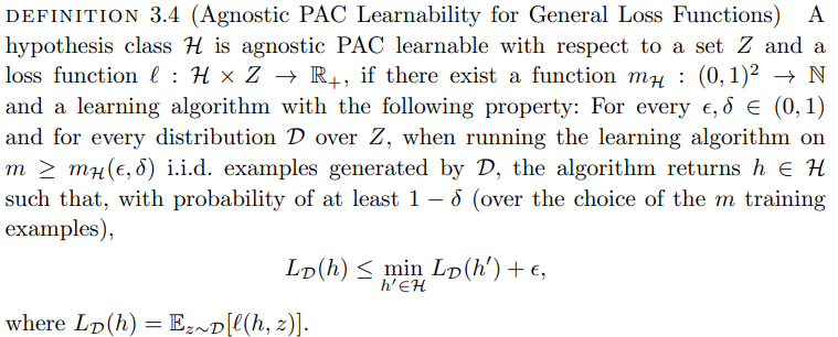
4: hitting the goalposts- finite hypothesis classes
Now that we have a clear criterion for acceptable learning algorithms (PAC learnability), we should alter our original ERM setup and check if we satisfy this criterion.
Note that since PAC learnability is a property of the chosen hypothesis class we’re trying to learn, we will only have to adjust the hypothesis class to which we apply the ERM algorithm.
The clear adjustment to make is a restriction of \(\mathcal{H}\) to the finite case, so that it does not include trivially bad functions like “memorize the sample set”. Intuitively, the bad “memorize” hypothesis we’re trying to avoid belongs to a family of functions which would require an infinitely long lookup table, and is thus excluded in the restriction to the finite case.
The question now is “does our first attempt, i.e. restricting \(\mathcal{H}\) to the finite case, actually give us that \(\mathcal{H}\)” is PAC-learnable? It turns out the answer is yes.
I’ll skip the proof, which you can read if you’re interested (roughly page 55 in the linked text), but the main idea is that by requiring \(|\mathcal{H}| \leq \infty\), we can use the union bound (\(P(A \cup B) \leq P(A) + P(B)\)) and Hoeffding’s inequality to get the following result:
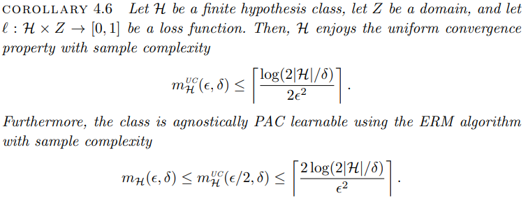
Here, \(m_{\mathcal{H}}\) is the minimum number of samples required to guarantee that our learning algorithm will be probably approximately correct.
Note that if we tighten our error tolerance (decrease \(\epsilon\)), tighten our confidence bound (decrease \(\delta\)), or increase the scope of our model (increase \(\mathcal{H}\)) we will need more samples to get the same guarantee.
In other words: a broad hypothesis class will require more samples than a narrow one to achieve good performance
5: quick recap
So far, this may feel very detached from reality, and it feels like all we’ve done is manipulate definitions, but we’ve actually uncovered two very deep truths from scratch:
- our standard learning paradigm will be minimizing loss on the training set
- a good way to avoid bad outcomes is to restrict the set of admissable models
Next, we will consider point 2 in more depth.
6: the bias-variance tradeoff
We have observed that restricting the size of \(\mathcal{H}\) can help in avoiding overfitting. The natural question remains: what are the drawbacks?
Well, our PAC definition gives us guarantees about ERM performance only with respect to the best possible model in our given hypothesis class: This is what is meant by the min of \(h'\) in the PAC statement \(L_\mathcal{D}(h) \leq \min_{h' \in \mathcal{H}} L_\mathcal{D}(h') + \epsilon\)
So we can think about the size of \(\mathcal{H}\) as follows. If we’re approaching a learning problem and have a fixed number of samples:
Large \(\mathcal{H} \implies\)
- increased risk of overfitting (recall the sample complexity bound obtained earlier)
- increased chance that some \(h \in \mathcal{H}\) will be able to model the true distribution
equivalently, a small \(\mathcal{H} \implies\)
- lower chance of overfitting
- higher chance that no model in \(\mathcal{H}\) will be powerful enough to model the true distribution
To line our observations up with standard terminology, we say:
Restricting \(\mathcal{H}\) (trading away model complexity) amounts to introducing inductive bias which:
- may increase the approximation error
- aka increases the loss of the best possible \(h \in \mathcal{H}\)
- our restriction may be so severe we can’t capture the essence of the true distribution
- may decrease the estimation error
- aka the difference between the loss on the sample vs the loss on the true distribution
- our restriction saves us from effectively memorizing the sample and losing predictive power
We call it inductive bias because it reflects the use of prior knowledge about the distribution to narrow our set of possible hypotheses and thus avoid higher sample complexity and overfitting risk, at the cost of robustness.
7: the no-free-lunch theorem
At this point, the only remaining question is “why not build a universal learner?”
We’ve shown that, in practice, introducing inductive bias can be a good strategy to approach learning problems, as it can alleviate the natural risk of overfitting to data, and reduce the amount of data we need to see.
I like to think of it as: modeling a low-entropy distribution with an overpowered model will naturally introduce noise, and modeling a high-entropy distribution with an underpowered model will naturally underperform.
However, we haven’t ruled out the possibility of a learner that solves every problem. If such a thing were possible, we should probably spend all our time on that, so it’s worth ruling it out.
There’s an often-cited theorem from Statistical Learning Theory that addresses this. From the text:
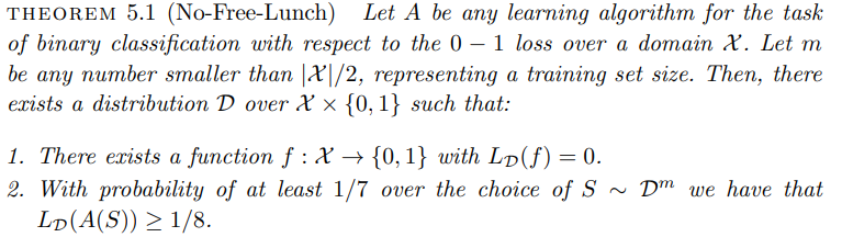
This is pretty opaque, so let’s consider the colloquial phrasing and go from there:
“This theorem states that for every learner, there exists a task on which it fails”
Seems pretty reasonable, but I think we can get a better intuition by rephrasing it, taking note of the fixed sample size in the definition. I’ll say instead:
“For any fixed, reasonable sample size from a domain \(\mathcal{X}\), no learner can guarantee high accuracy and confidence for all possible distributions \(\mathcal{D}\) over \(\mathcal{X}\)”
This seems more immediately believable to me, but we can do better by supposing it’s false and going by contradiction. Then we’d have that:
“For a fixed, reasonable sample size over a domain \(\mathcal{X}\), there exists a learner which gives arbitrarily good \((\epsilon, \delta)\) performance on every distribution \(\mathcal{D}\) over \(\mathcal{X}\).
This seems highly implausible, reinforcing the idea that no single learner can be optimal for all possible distributions. To understand this better, consider an analogous (though very loosely phrased) statement: ‘The uncertainty in any distribution \(\mathcal{D}\) can be fully captured by a smaller sample \(S\),’ or equivalently, ‘we can losslessly compress any data distribution.’ Clearly, this is false, as we cannot capture all the variability of any distribution in a finite sample without some loss of information.
I’m not going to go through the formal proof here, because it’s notationally cumbersome, but the core idea is pretty straightforward and you can see a sketch of it in this video.
That said, the intuitive proof-by-contradiction feels pretty solid, at least to me.
The elephant in the room is bascially the objection “wait, I feel like gpt4 is a pretty universal learner; it knows natural language which can express pretty much anything…”.
The counterpoint is that GPT-4 and similar models incorporate significant inductive biases in their architectures, (e.g. assumptions about token dependencies) which necessarily limit their universality across different types of data distributions. Just because the model has good real-life generalization capabilities does not mean it can accurately model literally every pathological distribution over token sequences.
8: conclusion:
If all of this theory feels useless, like we basically just played with definitions and notations, that’s OK. When we started, it wasn’t clear that we wanted to choose an inductive bias at all, or that minimizing the sample loss was the way to go, but hopefully now these feel like the natural and obvious things to do.
For advanced practitioners, this might feel silly, but I remember taking a grad-level machine learning course as an undergrad and was very confused at the start why we took such things for granted. Maybe others just see these as obvious, but I certainly had to spend a few days thinking about it. This writeup was done to clarify my own understanding of some of the basics of statistical learning.
optimization techniques
jan 19, 2026
recap
We’re working our way up to modern transformer-based language models, and we’ve covered the basics of how to approach learning in general.
The basic regime we’re following is:
- choose a sample \(S\) (training set) from the distribution we want to model
- choose a loss function \(\ell\) that measures prediction error
- choose a ‘hypothesis class’ (~model architecture) \(H\)
Then, we find a function \(h \in H\) which minimizes the empirical risk over \(S\).
optimization
Now we’re asking an optimization question. We’re just minimizing some objective function. And at this point, we don’t have any constraints on what the objective or loss functions look like.
This means we probably want to look for techniques which place minimal constraints on our objective function.
For instance, there are a bunch of EM-based procedures and bayesian frameworks for learning. With these, the idea is to pick some nice distribution as the hypothesis class, and use variations on the Expectation-Maximization algorithm to estimate its parameters. The problem there is that integrating your priors needs to be analytically tractable.
Even if we think of more classical optimization methods like ‘set derivative equal to zero and solve’, again we’re faced with analytical intractability. Other popular optimization algorithms include things like linear programming. But then the objective function needs to be linear and convex. And those are pretty stringent requirements that would make life extremely difficult.
Fortunately, there is an iterative optimization algorithm that only imposes one requirement: differentiability in the objective and loss functions.
gradient descent
First, it’s worth mentioning that the differentiability requirement does mean that we’re making another assumption on the functional form of our model.
Namely, that our model \(h_\theta : \mathbb{R}^n \to \mathbb{R}^m\) is differentiable with respect to its parameters \(\theta\). Before, we had no such restriction. This means that we’re going to have to convert our model inputs to real-valued vectors, and our loss function is also going to have to be differentiable.
Let’s say our model is \(h_\theta\) and our loss function for a single example is \(\ell(h_\theta(x), y)\) where \(y\) is the true label.
According to the ERM procedure, we need to minimize our average sample loss:
\[ L_S(\theta) := \frac{1}{N}\sum_{i=1}^{N} \ell(h_\theta(x_i), y_i) \;\; \text{for} \;\; (x_i, y_i) \in S \]
Gradient descent does this by setting, for some small ‘step size’ \(\eta\):
\[ \begin{align} \theta_0 &:= \text{random} \\ \theta_{t+1} &:= \theta_t - \eta \nabla_\theta L_S(\theta_t) \\ &= \theta_t - \frac{\eta}{N}\sum_{i=1}^{N} \nabla_\theta \ell(h_\theta(x_i), y_i) \bigg|_{\theta=\theta_t} \end{align} \]
In other words, we literally just follow the gradient around the loss landscape for some arbitrary number of iterations until we’re happy.
In python, a barebones implementation for a random function on \(\mathbb{R}^2\) looks like:
def gd(grad_fn, start, n_steps, stepsize):
    x, y = start
    for _ in range(n_steps):
        gx, gy = grad_fn(x,y)
        x -= stepsize * gx
        y -= stepsize * gy
    return x,y
worked example
Ok let’s pick a trivial example.
Consider the function \(f(x, y) = 1 +
\sin(x) + \cos(y) + \frac{1}{10}(y + y^2 + x^2)\). 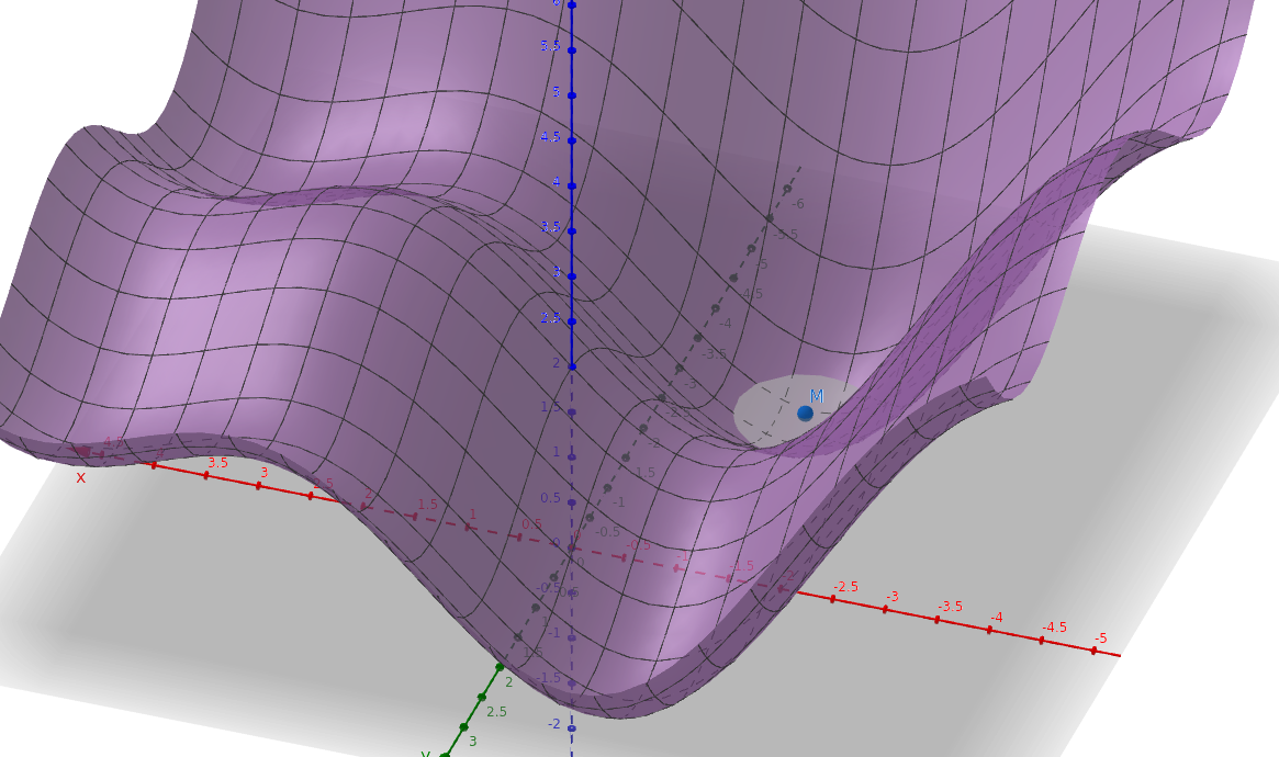
As you can see, we have a nice little example with some local minima to play with.
We can manually derive the gradient: \[ \nabla f(x, y) = \begin{pmatrix} \cos(x) + \frac{1}{5}x \\ -\sin(y) + \frac{1}{10} + \frac{1}{5}y \end{pmatrix} \]
# arbitrary function with some local minima
def f(x, y):
    return 1 + sin(x) + cos(y) + (1/10)* (y + y**2 +x^2)

# hand-derived gradient
def grad_f(x,y):
    grad_x = cos(x) + (1/5) * x
    grad_y = -sin(y) + 1/10 + (1/5) * y
    return grad_x, grad_y

# hand-derived analytical solution
def f_argmin():
    return -1.32, -2.68
By manual ‘set-derivative-equal-to-zero’ method we know the solution should be around \((-1.32, -2.68)\)
Does gradient descent work? …
(ml2) ❄️ ~/projects/ml2/ml2 λ python main.py
gd(0, 0) => (-1.31,-2.69)(True) w/ stepsize=0.01 in 1000 steps
gd(4, 2) => (3.84,2.50)(False) w/ stepsize=0.01 in 1000 steps
Sometimes! But we get trapped in local minima.
You can imagine the procedure as hill descending. Like a ball. But our ball has no momentum.
What if we add some? By that, I mean literally add a velocity term \(\mu\), where we just carry over some of the previous gradient information to the present iteration:
\[ \begin{align} \theta_0 &:= \text{random} \\ v_0 &:= 0 \\ v_{t+1} &:= \mu v_t + \eta \nabla_\theta L_S \\ \theta_{t+1} &:= \theta_t - v_{t+1} \end{align} \]
In code:
# gd with momentum (sutskever version)
def momentum(grad_fn, start, n_steps, stepsize, mu):
    x, y = start
    vx, vy = 0,0
    for _ in range(n_steps):
        g = grad_fn(x,y)
        vx = mu * vx + stepsize * g[0]
        vy = mu * vy + stepsize * g[1]
        x -= vx
        y -= vy

    return x, y
Does this version work?
(ml2) ❄️ ~/projects/ml2/ml2 λ python main.py
momentum(0, 0) => (-1.30,-2.68)(True) w/ stepsize=0.01 in 1000 steps
momentum(10, 10) => (-1.30,-2.69)(True) w/ stepsize=0.01 in 1000 steps
Yes …
We can also see the convergence plots. I.e., how far away from the optimum are we at each step of gradient descent? For standard GD and the momentum version:
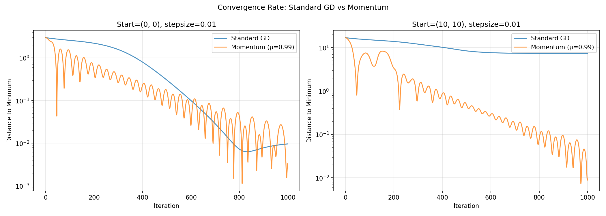
Its funny the extent to which the convergence plot follows physical intuition. As an aside, you can prove properties about convergence (usually limited to L-smooth convex functions) using an ODE dual formulation with physics-like position and velocity components. That’s for a followup (if ever) though.
Also, I lied earlier.
(ml2) ❄️ ~/projects/ml2/ml2 λ python main.py
gd(0, 0) => (-1.31,-2.69)(True) w/ stepsize=0.01 in 1000 steps
gd(4, 2) => (3.84,2.50)(False) w/ stepsize=0.01 in 1000 steps
momentum(0, 0) => (-1.30,-2.68)(True) w/ stepsize=0.01 in 1000 steps
momentum(4, 2) => (3.84,2.50)(False) w/ stepsize=0.01 in 1000 steps
Because the function I chose is actually pretty pathological and nasty, we can still pick starting points where momentum sgd fails to converge to the global optimum.
So. Yeah it’s not foolproof.
gradient computation, sgd
In our toy example, we literally just optimized an arbitrary function.
In reality, in a real optimize-the-model scenario, we are optimizing parameters, and we’re computing the average gradient- i.e. not just at one point, but at all the points in the sample set.
The problem with this is that it becomes computationally intractable at large sample sizes.
The solution is to just compute the average over a small batch of samples. This is called stochastic gradient descent and is the real one people use in practice.
better versions
One improvement is called the nesterov method where instead of computing the gradient at the current weights \(\theta_t\) you compute the next gradient at a lookahead point \(\theta_t - \mu v_t\).
This is nice because if your loss landscape is brutal (ratio of smallest to largest eigenvalue of the hessian is really high), the lookahead version cancels some of the oscillation that would happen.
Other popular variants like adamW adjust hyperparameters in smarter ways than just “keep the learning rate the same the whole time”.
I might do a followup post on adamW but for now we have a good enough tool.
model architecture
Jan 22 2026
Last time we introduced gradient descent. Now we ought to choose a model architecture.
Of course, it’d be absurd to try and pick a full model architecture at this point. We don’t have any empirical data. We have a few a priori notions about some broad theoretical ideas. That’s it.
However, if you recall from last time, our hand is at this point already somewhat forced:
we’re making another assumption on the functional form of our model. Namely, that our model \(h_\theta : \mathbb{R}^n \to \mathbb{R}^m\) is differentiable with respect to its parameters \(\theta\).
Also it’s worth typechecking the model input/output quickly. Recall we’re trying to model language so we have something like:
\[ \text{text} \xrightarrow[\text{?}]{} \begin{pmatrix} x_1 \\ \vdots \\ x_n \end{pmatrix} \xrightarrow[f_\theta]{} \begin{pmatrix} y_1 \\ \vdots \\ y_m \end{pmatrix} \xrightarrow[\ell]{} \mathbb{R} \]
So now the question is… which functional form should \(f_\theta\) take?
Let’s think about our criteria, in order of most to least important:
- differentiable
- expressive; can approximate arbitrary (reasonably nice) functions
- efficiently computable, numerically stable
- works well with vectorized input
any guesses?
the original universal approximation theorem
At this point, at least for me, the following theorem jumps to mind:
Stone-Weierstrass Approximation Theorem: Suppose \(f\) is a continuous real-valued function defined on the real interval \([a, b]\). For every \(\epsilon > 0\), there exists a polynomial \(p\) such that for all \(x\) in \([a, b]\), we have \(|f(x) - p(x)| < \epsilon\)
In other words, polynomials fit the bill pretty well. So that’s the solution then, right? just stack polynomials?
But then like… how would we do that? Something like:
\[ f_i(x_i) = a_0 + a_1 x_i + a_2 x_i^2 + \dots + a_n x_i^n \]
This looks reasonable but also it doesn’t really fit our criteria:
- ✅ polynomials are definitely differentiable
- ✅ polynomials can approximate most functions we care about
- ❌ high degree polynomials are extremely numerically unstable, and no hardware-level support
- ❌ component-wise evaluation is ugly, we lose a lot of information
So we’re close, but not quite.
What about if we formulated the polynomial with cross terms:
\[ f(x_1, \dots, x_n) = \sum_{k_1 + \dots + k_n \leq d} a_{k_1 \dots k_n} x_1^{k_1} \cdots x_n^{k_n} \]
Well ok so if we did this, we don’t ‘lose information’ but now we have a parameter explosion; estimating parameters there is \(O(n^d)\)… grossly inefficient. So that’s really no help. We’re still only hitting half our criteria.
mlp universal approximation theorem
Fortunately, it turns out there’s another family of functions that does satisfy these criteria: chained compositions of affine linear transformations and nonlinear ‘activation’ functions:
\[ \sigma(W_2 \cdot \sigma(W_1 x + b_1) + b_2) \]
where \(W \in \mathbb{R}^{m \times n}\), \(b \in \mathbb{R}^m\), and \(\sigma\) is a non-polynomial continuous function (e.g. sigmoid, ReLU).
You’ve probably heard of these. We call them MLPs (multilayer perceptrons). You’ve probably seen the classic image (which personally I find misleading and ugly compared to the symbolic form but whatever):

And, fortunately, it turns out we have theorems proving that functions of this form are able to approximate reasonably ‘nice’ functions.
There are various forms of the theorem for various levels of ‘nice’ function (continuous, lebesgue integrable, continuously differentiable, etc…) and different nonlinear activations \(\sigma\).
I’m not going to prove the theorem here, but the basic idea is this (wlog, for dim=1):
- use weighted sums of expressions of the form \(\sigma(ax +b)\) to produce stairsteps
- combine the stairsteps to fit your function
- increase the number of stairsteps arbitrarily a la riemann integration
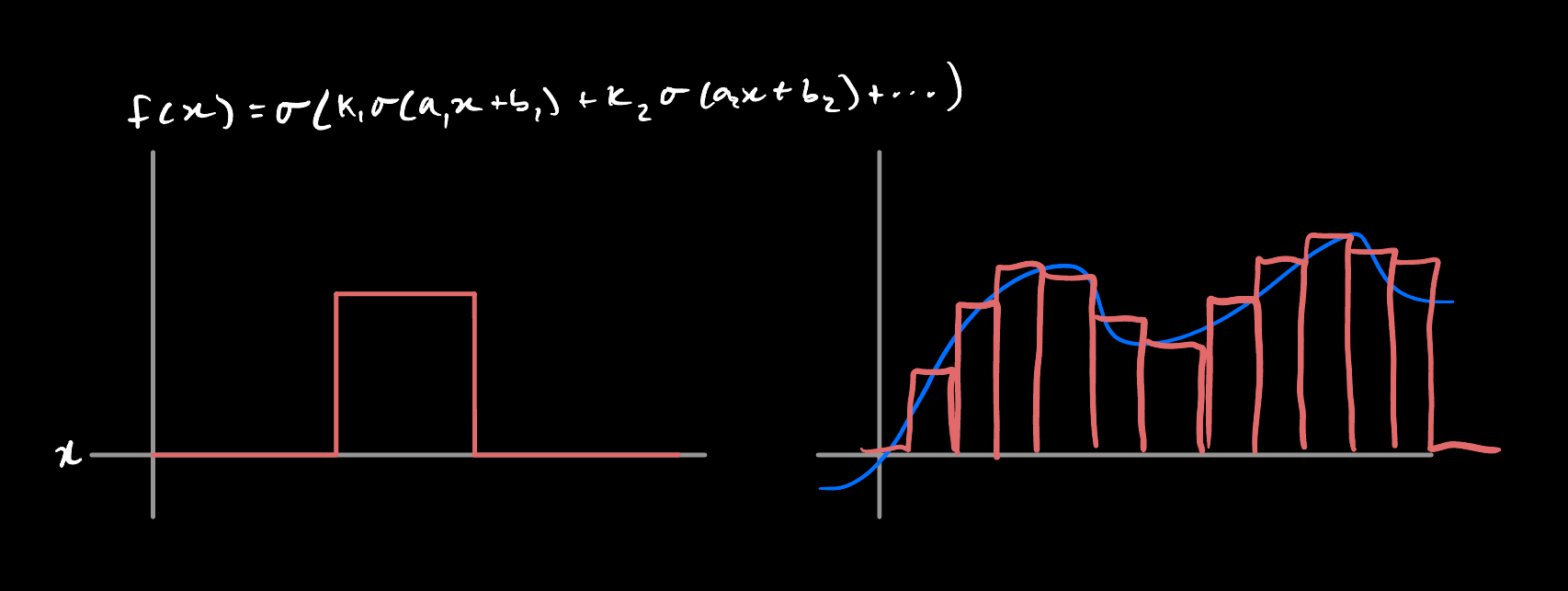
This site has a pretty solid explainer if you want more depth, but they use a nonlinearity of the form \(\sigma = (1+e^{-x})^{-1}\), i.e. the classic sigmoid.
But we’re building up from scratch and it’s not clear why we’d choose that nonlinearity.
Fortunately some of those approximation theorems also work for the dumbest possible nonlinearity, the ReLu (rectified linear unit) function:
\[ \mathrm{ReLu}(x) := \mathrm{max}(0, x) \]
And instead of stairsteps, the visual proof intuition is more like jagged peaks, since the ReLu function technically isn’t sigmoidal (it goes off to \(+\infty\)).
You can spend 15 minutes in desmos to grok the intuition if you aren’t sold.
recap
Let’s make sure our new candidate functional form actually checks our boxes:
- ✅ affine linear transformations and relu are differentiable (x=0 is measure 0 so just be a good little engineer and pretend that max function is differentiable at zero with derivative 1 or 0 depending on your preference)
- ✅ we have universal approximation theorems saying we can approximate lots of functions
- ✅ the computation here boils down to matmul, and hardware acceleration for this is a trillion dollar industry
- ✅ this trivially plays nice with vector inputs, with managable layer-wise computational complexity \(O(m \times n)\) for \(W \in \mathbb{R}^{m \times n}\)
Great!
I’ve gone kind of fast so here’s the new picture:
One Layer: \[ \text{text} \Rightarrow \begin{bmatrix} x_1 \\ x_2 \\ \vdots \\ x_n \end{bmatrix} \xrightarrow{L_1} \begin{bmatrix} \sigma(w_{11}x_1 + w_{12}x_2 + \cdots + w_{1n}x_n + b_1) \\ \sigma(w_{21}x_1 + w_{22}x_2 + \cdots + w_{2n}x_n + b_2) \\ \vdots \\ \sigma(w_{m1}x_1 + w_{m2}x_2 + \cdots + w_{mn}x_n + b_m) \end{bmatrix} = \sigma(Wx + b) \]
N layers:
\[ \text{text} \Rightarrow \mathbb{R}^n \xrightarrow{L_1} \mathbb{R}^m \rightarrow \cdots \rightarrow \mathbb{R}^k \xrightarrow{L} \mathbb{R} \]
So at this point, here’s what we have left to do before we can start doing language modeling:
- figure out what loss function to use
- get some data to test on
- figure out how to encode the data into euclidean space
- decide hyperparameters; how wide should the network be? sgd learning rate? etc…
Next time we’ll look at loss functions!
choosing a loss function
Jan 22, 2026
Quick recap up to now:
We’re trying to do language modeling. We know that we’re converting text samples into elements in \(\mathbb{R}^n\), and operating on them with differentiable functions (MLP layers for now), so that our optimizer machinery works.
What’s next?
Well, we want our network to take in some chunk of text, \([t_1, t_2, \dots, t_n]\), and predict the most likely next piece of text \(t_{n+1}\).
What this means is that our model output should be a vector which represents the probabilities of each chunk appearing next in the input sequence. It’s kind of the only reasonable way to make this work.
For example, given the input “the quick brown fox jumps over the lazy”, we want our model to output something like:
\[ \begin{bmatrix} \text{rabbit} \\ \text{fox} \\ \text{green} \\ \text{eliezer} \\ \text{dog} \\ \text{the} \\ \text{SPACE} \end{bmatrix} \to \begin{bmatrix} 0.02 \\ 0.05 \\ 0.01 \\ 0.00 \\ 0.82 \\ 0.03 \\ 0.07 \end{bmatrix} \]
probability conversion
OK first we have a problem. You’ll note that above the probabilities sum to one, and each probability is in the range \((0,1)\). However, we have zero guarantee (and we should not expect) that the network will magically output a vector containing such a valid probability distribution.
So first we need to pass it through a (differentiable) function that fixes this.
First we need to fix the negatives. We probably also want a monotonically increasing function for self-explanatory reasons. The obvious choice is the exponential function.
But then of course we don’t have a valid “summing-to-one” vector and the components can be arbitrarily large.
And again the obvious fix is just to normalize it. I.e. divide each component by the sum of all the components. And so all together we have:
\[ \mathrm{validated}(x)_k := \frac{e^{x_k}}{\sum_{i=1}^n e^{x_i}} \]
And we don’t call it the ‘validated’ function, we call it ‘softmax’. It’s the obvious “make-it-a-real-probability-distribution” function.
loss function choices
Great ok so now we have a nice differentiable function we can throw on the end of the model to end up with a real probability distribution.
Now we need a measure of “how close to the real distribution is this?”
First, note that when we train this on text samples, the “real distribution” for any given piece of text will just be a “one-hot” vector, or a standard basis vector. This is because it’s true that with probability 1 we actually did observe in the training set that this particular piece of text ended in this particular way.
I think you could probably formulate it another way but honestly this really is the most straightforward so i’m going to hope you just buy this.
So the “true distribution” might look like this:
\[ \begin{bmatrix} \text{rabbit} \\ \text{fox} \\ \text{green} \\ \text{eliezer} \\ \text{dog} \\ \text{the} \\ \text{SPACE} \end{bmatrix} \to \begin{bmatrix} 0.00 \\ 0.00 \\ 0.00 \\ 0.00 \\ 1.00 \\ 0.00 \\ 0.00 \end{bmatrix} \]
Let’s call our model prediction \(\hat{y}\) and our true reference output \(y\), both in \(\mathbb{R}^n\).
Recall that we’re trying to minimize loss, so we want to assign large numbers to bad predictions and small (or large, negative) numbers to good predictions.
Immediately we have a strong candidate: the naive dot product, negated. i.e. \(l(\hat{y}, y) = - \langle \hat{y}, y \rangle\).
I say ‘immediately’ because the geometric intuition is solid. If our \(\hat{y}\) is totally orthogonal to \(y\) then we get a zero. If \(\hat{y} = y\) then we get \(-1\). Great.
Consider the scenario for the following three guesses, \(a\), \(b\), and \(c\), against an observation \(y\):
\[ \begin{aligned} y &= [1, 0] \\[0.5em] a &= [0.1, 0.9] \implies \ell = -0.1 \\ b &= [0.5, 0.5] \implies \ell = -0.5 \\ c &= [0.9, 0.1] \implies \ell = -0.9 \end{aligned} \]
So it looks like this function works as a loss function for our problem.
The thing is, no one uses it. Why?
cross entropy loss
The version of this “multi-class classification” loss function you’ll actually see is this:
\[ l(\hat{y}, y) = -\langle \log(\hat{y}), y \rangle = -\sum_{i=1}^n \log(\hat{y}_i) y_i \]
The function is known as cross-entropy loss (CEL).
Note this simplifies to \(\mathrm{CEL}(\hat{y}, y) = -\log(\hat{y}[\mathrm{true index}])\) in the one-hot case.
So why the log? A few reasons.
First: theoretical soundness.
There’s this notion of “entropy” as a quantity which (roughly speaking) measures the uncertainty in a probability distribution. higher entropy = more bits required to ‘describe’ the distribution.
it’s written \(H(p) = - \sum_{i=1}^n p_i \log(p_i)\).
Basically if we just use cross-entropy we get a nice theoretical interpretation of what we’re doing.
The big payoff there is that we can say that minimizing cross-entropy loss is the same as doing MLE for categorical distributions, and that minimizing cross-entropy is equivalent to minimizing KL divergence.
There’s a wealth of resources out there to learn more about the theoretical justifications here. Shannon’s original information theory paper is very digestible and worth reading.
For the sake of this blog post I’m not going to dwell on these facts now, although it definitely is worth a followup at some point. I don’t want to undersell the importance of this theoretical connection, but I think we can reach a minimum viable justification of why we use cross-entropy without a statistical digression at this point in the series.
Second: practical considerations:
consider the same scenario but with our new cross-entropy loss function.
\[ \begin{aligned} y &= [1, 0] \\[0.5em] a &= [0.1, 0.9] \implies \ell = 2.30 \\ b &= [0.5, 0.5] \implies \ell = 0.69 \\ c &= [0.9, 0.1] \implies \ell = 0.11 \end{aligned} \]
Let’s compare this to earlier, using the “confidently correct (c) case as a baseline”
negative dot product loss penalty for being:
- uncertain: ~5x baseline
- confidently wrong: ~9x baseline
cross-entropy loss penalty for being:
- uncertain: ~6x baseline
- confidently wrong: ~21x baseline
Clearly introducing the logarithm has made our loss landscape far more expressive. The hope is that this will give our network a stronger gradient signal when we’re confidently wrong, which is when it’s most needed.
It’s also worth mentioning that doing the softmax exponential function and then taking a logarithm can be exploited by popular ML frameworks like pytorch to improve numerical stability.
Also, this formulation makes the gradient of the loss look really nice. if we set \(z = f_\theta(x)\), then:
\(\nabla_z \mathrm{CEL} = \mathrm{softmax(z)} - y\)
If you don’t buy the theoretical reasons, the practical considerations are probably good enough to accept that CEL is the right loss function to choose.
perplexity
One annoying thing about the loss function is that it’s sort of unitless. Technically not really, we could say like “nats” or “bits” but it’s not easy to interpret.
The way out of this is to use a measure called perplexity, defined as:
\[ \mathrm{perplexity} = e^{\mathrm{CEL}} = e^{-\log(\hat{y}_i)} = \hat{y}_i^{-1} \]
Where \(i\) is the index of the true
label. The theoretical interpretation is that a perplexity of e.g. 10
means that your model is equally split between choosing 10 options. It’s
more meaningful in the non-degenerate non-one-hot case but whatever.
It’s the number you want to go down when you stack a bunch of layers and
hit model.train.
next steps
Ok! At this point we have some basic procedure for learning established, we’ve got our optimization technique of choice, have a reasonable functional form for our first models, and now a loss function.
Next up, it’s time to test this stuff in practice!
shakespeare mlp test run
jan 24 2026
Ok so at this point we have most of what we need train our own primitive language model.
Specifically, we’re going to build and train an MLP network on on the complete works of shakespeare, about 5 MB of text.
To get a baseline, I had claude cook up a quick ngram model for a baseline.
Because of what we said about overfitting earlier, the standard procedure here is to train the model on most of the text (80-90%) and save the rest for testing. We don’t want to test the model on stuff it’s already seen; pretty straightforward.
The results of the ngram are:
ngram dataset
- Train: 4,273,149 chars
- Val: 1,086,193 chars
- Vocab: 97 unique characters (includes curly quotes, em-dash, some French/Latin accented chars)
Perplexity & Accuracy
| n | Train PPL | Val PPL | Train Acc | Val Acc | Contexts |
|---|---|---|---|---|---|
| 2 | 12.35 | 12.29 | 26.0% | 26.7% | 100 |
| 3 | 6.93 | 7.87 | 40.4% | 38.5% | 2,341 |
| 4 | 4.92 | 5.88 | 49.0% | 47.0% | 20,634 |
| 5 | 3.99 | 5.46 | 55.1% | 51.5% | 98,493 |
| 6 | 3.48 | 6.21 | 59.3% | 51.9% | 309,366 |
5-gram is the sweet spot. At 6-gram, val perplexity increases (overfitting to training contexts).
Generation Samples
(5-gram, temperature=0.8)
“Enter”
Enter Caesar said the country many outward's scene II. And his dead; for that
with your him like not please in the done abused, thee are not from his power
Into France.

HORTENSIO.
This valoursed by the did so prattle of his about of men disdainter they'll
for throat we were is somethink your commonweal w
“Shall”
Shall of our some thou take thy life the was a man this one this,
Come, let sir, I am all seeks, and danger bottle, have doubless so in that
I am much,
Unless his but let me of him to my soul's since in since to be the thou the rams
Pink on the are so thee a cart good consieur; and such combine,
And, but
Notes
- Model uses add-k smoothing (k=0.01)
- Generation degrades when it samples rare characters (French/Latin accented chars like é, æ, œ) because contexts become unseen
- Captures basic structure: character names, stage directions, dialogue format, approximate meter
- Grammar is mostly nonsense but locally plausible
MLP time
Ok so the n-gram is pretty good. Time to see if we can beat it on shakespeare with our MLP.
And at this point the one thing we haven’t covered is how we encode text. For comparison with the n-gram, and since it’s a clear starting point, we’re going to predict text character by character.
To do this, we first get all the characters in the training set:
def create_vocab(corpus: list[Path], vocab_path: Path) -> dict[int, str]:
    char_set = set()
    for file_contents in corpus_iter(corpus):
        char_set.update(set(file_contents))

    vocab = {i: c for i, c in enumerate(list(char_set))}
    with open(vocab_path, 'w') as f:
        json.dump(vocab, f)
        print(f'saved vocab json to {vocab_path}')

    return vocab
So now each character is representable as a digit. The obvious problem is that if we have that \(a = 1\), \(b = 2\), and \(c = 3\), the relationship \(1+2=3\) is meaningful but in language-world, \(a+b=c\) is not.
The way to fix this is to give each character it’s own unique direction in an ‘embedding space’.
I.e. the \(j^{\mathrm{th}}\) character in our dataset corresponds to the one hot or standard basis vector \(e_j\) in \(\mathbb{R}^d\) where \(d:=\text{vocab size}\).
Theoretically, that’s all there is to it.
However, for practical (computational) reasons, we don’t actually use these one-hot encodings. We just use the character index, and feed them into an ‘embedding’ layer, before passing them into the rest of the network.
self.embedding = nn.Embedding(len(vocab), emb_dim)In other words, the embedding layer has type \(\mathbb{Z} \to \mathbb{R}^d\), which is identical to converting to a one-hot encoding \(\{0,1\}^d\) and passing it through a linear layer with no bias. (no bias because \(xW +b\) where \(x\) is one-hot means you get \(W[i] +b\) for token \(i\), and this constant \(b\) can just be absorbed into the weight matrix)
The rest of the network is fairly straightforward, since we just have linear layers and relu to play with.
We’ll start with:
h_size = emb_dim * ctx_len
nn.Sequential(
    nn.Linear(h_size, h_size),
    nn.ReLU(),
    nn.Linear(h_size, len(vocab))
)
And the training loop is just boilerplate for our optimizer with some logging:
def train(model: nn.Module,
          optimizer: optim.Optimizer,
          train_loader: DataLoader,
          val_loader: DataLoader,
          logger: logging.Logger,
          device: torch.device,
          batch_log_interval: int=0,
          batch_val_interval: int=0):

    log_train_info(model, train_loader, logger)
    loss_fn = nn.CrossEntropyLoss()
    model.to(device)
    model.train()

    n_batches = len(train_loader)

    if batch_log_interval == 0:
        batch_log_interval = n_batches // 10
    val_loss = 0

    if batch_val_interval == 0:
        batch_val_interval = batch_log_interval * 2

    for batch_no, batch in enumerate(train_loader):
        batch_t0 = time.perf_counter()
        batch = batch.to(device)
        x = batch[:, :-1]
        y = batch[:, -1]
        y_pred = model.forward(x)

        loss = loss_fn(y_pred, y)
        optimizer.zero_grad()
        loss.backward()
        optimizer.step()

        if (batch_no+1) % batch_val_interval == 0:
            val_loss = validate(model, val_loader, device)

        if (batch_no+1) % batch_log_interval == 0:
            log_batch(logger, loss.item(), val_loss, batch_no + 1, batch_t0, train_loader)

    final_val_loss = validate(model, val_loader, device)
    logger.info(f"training finished w/ final val ppl={math.exp(final_val_loss)}\n\n")
    return final_val_loss
running the MLP
There are a few ‘hyperparameters’ that we haven’t set yet. We’ll just kind of pick random ones to start:
context_length=10   # how many chars does the network see at once
batch_size=1024     # how many samples do we compute at once on gpu
lr=0.01             # learning rate (step size) for sgd
momentum=0.9        # momentum coefficient for sgd
n_layers=2          # how many layers in our MLP
emb_dim=64          # output dim of the first implicit (embedding) layer
hidden_dim=64*10    # subsequent layer dimensions; (emb_dim * context_length)
Let’s run it and see how we do:
 batch 250/4711; 'train_loss': 2.617, 'train_ppl': 13.694, 'val_loss': 0, 'val_ppl': 1.0}
 batch 500/4711; 'train_loss': 2.262, 'train_ppl': 9.603, 'val_loss': 0, 'val_ppl': 1.0}
 batch 750/4711; 'train_loss': 2.215, 'train_ppl': 9.166, 'val_loss': 0, 'val_ppl': 1.0}
 batch 1000/4711; 'train_loss': 2.2, 'train_ppl': 9.025, 'val_loss': 0, 'val_ppl': 1.0}
 batch 1250/4711; 'train_loss': 2.133, 'train_ppl': 8.437, 'val_loss': 0, 'val_ppl': 1.0}
 batch 1500/4711; 'train_loss': 1.999, 'train_ppl': 7.384, 'val_loss': 0, 'val_ppl': 1.0}
 batch 1750/4711; 'train_loss': 2.04, 'train_ppl': 7.69, 'val_loss': 0, 'val_ppl': 1.0}
 batch 2000/4711; 'train_loss': 1.894, 'train_ppl': 6.649, 'val_loss': 2.039, 'val_ppl': 7.684}
 batch 2250/4711; 'train_loss': 1.919, 'train_ppl': 6.817, 'val_loss': 2.039, 'val_ppl': 7.684}
 batch 2500/4711; 'train_loss': 1.95, 'train_ppl': 7.031, 'val_loss': 2.039, 'val_ppl': 7.684}
 batch 2750/4711; 'train_loss': 1.869, 'train_ppl': 6.48, 'val_loss': 2.039, 'val_ppl': 7.684}
 batch 3000/4711; 'train_loss': 1.821, 'train_ppl': 6.176, 'val_loss': 2.039, 'val_ppl': 7.684}
 batch 3250/4711; 'train_loss': 1.779, 'train_ppl': 5.927, 'val_loss': 2.039, 'val_ppl': 7.684}
 batch 3500/4711;'train_loss': 1.802, 'train_ppl': 6.064, 'val_loss': 2.039, 'val_ppl': 7.684}
 batch 3750/4711; 'train_loss': 1.867, 'train_ppl': 6.472, 'val_loss': 2.039, 'val_ppl': 7.684}
 batch 4000/4711;71, 'train_loss': 1.732, 'train_ppl': 5.65, 'val_loss': 1.885, 'val_ppl': 6.585}
 batch 4250/4711;'train_loss': 1.879, 'train_ppl': 6.546, 'val_loss': 1.885, 'val_ppl': 6.585}
 batch 4500/4711; 'train_loss': 1.852, 'train_ppl': 6.376, 'val_loss': 1.885, 'val_ppl': 6.585}
 training finished w/ final val ppl=6.404950198477691
Not terrible! final perplexity of 6.4, so we’re close behind our highly inductively biased n-gram! And it’s worth noting our model is ingesting 10 characters at once; double the ‘context’ of the n-gram.
text generation:
One thing that’s worth noting before we look at the sample generations… There are many ways we could sample from the model output!
One way (“temperature zero”) is to just pick the biggest “logit” (thing that the model spits out at the end of the network before we softmax into probabilities for the loss function)
Another way is to scale up the logits by a constant in the softmax, and do multinomial sampling:
\[ \mathrm{softmax}(x,T) = \frac{e^{x_i / T}}{\sum e^{x_j/ T}} \]
where \(T\) refers to the ‘temperature’
sample generations, temperature = 0.2:
constrain and a stremant the with the stranger the word of the prother to the sure of the poor
her love to the words the words that have the word when and man the will be a the earth,well
shall not a strain the ward of the come..lord, and the with the are are the
Not bad! There’s some primitive broken grammar, legible words, etc…
Here’s a model generation for another run at a higher temperature:
“By fair and dorn-ooking.maye’d pergate,standed is to ming ahis fighty fropose,”
Also it’s worth noting that on this re-run, we finished with a val
ppl of 6.33. a full tenth of a point better than our
original run, even though nothing changed except the demo settings at
the end… SGD is definitely stochastic!
training dynamics
One other thing to note is that we’re still improving on the validation perplexity… and one advantage we have over the n-gram model is we can just… train more times on the same corpus and keep feeding more gradient information to our optimizer.
Let’s try it with a few ‘epochs’ (iterations on the same training set):
After a few epochs, we get a final val perplexity of
5.39, beating the 5-gram baseline!
Sample generations:
the more than the court the common the too love the common the common and the lives a p
the common and the content to the state and the charge of the time of the comes the commo
the heart of the court the rest the court the part of the common the common the common a
Except … the generation quality really sucks.
hyperparameter adjustment
Now it’s time to adjust some hyperparameters and see if we can’t improve the baseline:
Adjustment #1: longer context window:
Result: final ppl of 5.53 after 4 epochs.
Sample generations:
by all men’s judgements,if the shall be for the langer of the wine of the hands..say the seart of
minds,therefore are the comes of faith,they have love the heart of the stay and the forthhave
Dost thou hear, Camillo,can the reason of the state of the heart of the field.III. The same. A
Better! except now the model has 4.4M params instead of 400k. Training takes longer, but not 10 times longer thanks to gpu i guess.
Adjustment #2: wider network
This time we set hidden_dim = h_size + 40 (arbitrary
number)
Result: final ppl of 5.53 after 4 epochs.
Sample generations:
ot so.am as ignorant in that hath made of this from the sentle to the street,stard shall see his but a mounter str
basses, but oneamongst and so the death.TOBY.shall be my lord, and the shall be the stronged and str
ayers urgeth stillUnder what thou art thou shall be the willshe will be the hath of the world,therefore th
Adjustment #3: deeper network
This time we add another layer:
layers = [
    nn.Linear(h_size, h_size + k),
    nn.ReLU(),
    nn.Linear(h_size, h_size + k),
    nn.ReLU(),
    nn.Linear(h_size + k, len(vocab))
]
Result: final ppl of 5.13 after 4 epochs.
Sample generations:
rio, whom your gentle daughter here,there is the sealth of the man.II. The same. A Room in the Ca
us lawfully, or business;the emperor the course of the common the state the court of the state of the place of th
.—Fairest Emily,gods by the time of the course of the streets the present the heart of the present to the metter.[
Adjustment #3: wider and deeper network
this time we use the extra layer and have a wider layer, same as in #2.
Result: final ppl of 5.14 after 4 epochs.
Sample generations:
maculate, look on thy virgin;then the prince of the like and courtesy..am an and then, in
mportance, ’twerepiteous to the court of the wind of the world,he is not the common in the street on the like
ight.sighs resound through the rest of the state,when the higher that he will be the will have me, and therefore
Adjustment #4: layer gluttony
Ok so last result was really good what if we stack more layers and add more context?
context_length = 64
h_size = emb_dim * ctx_len
k = 80
layers = [
    nn.Linear(h_size, h_size + k),
    nn.ReLU(),
    nn.Linear(h_size + k, h_size + k),
    nn.ReLU(),
    nn.Linear(h_size + k, h_size + k),
    nn.ReLU(),
    nn.Linear(h_size + k, len(vocab))
]
It’s worth noting that the weight matrices scale quadratically… Each
weight matrix is on the order of context_length * emb_dim
squared parameters… so at these context lengths that’s ~52M
parameters.
Result: final ppl of 5.22 after 4 epochs.
Sample generations (temperature = 0.5):
PROMPT:  " shall not come about her,\nAway with him, and let her sport hers"
OUTPUT:  ".\n\nCASSIUS.\nWho, you are do read and him with the danger.\n\nFIRST LORD.\nI thou didst thee with this not shall be even and of his wing'st there,\nAnd this shall shall be so much father's the devinest, an"

PROMPT:  "es,\n    So mild, that patience seemed to scorn his woes.\n\nIn him"
OUTPUT:  " that the spiton of this daughter,\nBut with the world the thrive the strong under\nAnd predition of all the legged them their pleased,\nStand the properations and his more the nature.\n\nGLOUCESTER.\nWhat "

PROMPT:  "sk the spotted princess how she fares.\n\nShe says her subjects wi"
OUTPUT:  "th the bright of her be my delivery.\n\nARGANDREY.\nI will not not him to the storest,\nAnd therefore commanded.\n\nPANDARUS.\nNo, my lord, the country time.\n\nGLOUD.\nNo, not thou didst you seek you that me t"
Sample generations (temperature = 0.2):
PROMPT:  " about, let them depart.\n\nLEONTES.\nProceed:\nNo foot shall stir.\n"
OUTPUT:  "\nALLIA.\nNow now, my lord.\n\nPATRO.\nWhy, that I have seen the street the greater the sure of the find.\n\nPRINCE.\nWhy, then the strange of the blood, and so the time.\n\nLUCENTIO.\nI have not the time of the"

PROMPT:  "her trust her.\nFor every inch of woman in the world,\nAy, every d"
OUTPUT:  "eath the sing of my such as the\nThat he shall be a head the stand of the street\nThe strange that where they shall be the street\nThat the should be the beggard the eyes shall be so himself,\nAnd bring t"

PROMPT:  "roving.\nMy will is strong, past reason's weak removing.\n    Who "
OUTPUT:  "should be so much the heart of me,\nAnd with the town of the with the strong of the world,\nAnd then the time of the world so be the street.\n\nBRUTUS.\nI have not the world be that he would not have thee "
Adjustment #5: adjust the learning rate
Setting lr=0.001 yields a final val ppl of
8.6 and substantially degraded output. Possible this is
fixable by just letting it run longer, but training time is already long
enough already for 5mb of text input.
Setting lr=0.1 gets validation perplexity down to
4.979 before overfitting all the way back to
6.01. But even then the generation quality is pretty good…
Let’s check what happens if we stop before overfitting at 2 epochs:
Final val ppl of 4.91, and the sample generations are
quite good!
main | INFO | 2026-01-24 17:12:38 | Sample generations (temperature = 0.5):
PROMPT:  ' your bare words.\n\nSILVIA.\nNo more, gentlemen, no more. Here com'
OUTPUT:  'es the sea and my father was\nwith you are the next. I shall not say,\nMy brace the name of soon to the great still;\nAnd I you of all hangs and the three the sad,\nAnd as my banished to the brought and g'

PROMPT:  'emove.”\n\n“Ay me,” quoth Venus, “young, and so unkind!\nWhat bare '
OUTPUT:  'what we strings with the great so fast.\n\nCAESAR.\nAy, and the siege, let him in the sun by me?\n\nBRUTUS.\nWhy shall the first which return you there?\n\nMARCUS.\nWhy, sir, I shall be how thee shall be that '

PROMPT:  'mercy, Theseus. ’Tis to me\nA thing as soon to die as thee to say'
OUTPUT:  ' to you.\n\nSECOND CITIZEN.\nMy lord, I will; and you well as I not gate.\n\n [_Exit Dost that will in a man is storn.\n\nKING EDWARD.\nWhat a fair within. He will me, there of the sun the wingst a court.\n\nEn'
The above output came from a smaller network, so let’s bump up the depth/width and try again.
main | INFO | 2026-01-24 17:17:22 | training finished w/ final val ppl=4.694544337616929

main | INFO | 2026-01-24 17:17:22 | Sample generations (temperature = 0.5):
PROMPT:  'res; he hears, and nods, and hums,\nAnd then cries “Rare!” and I '
OUTPUT:  'have not with thee.\n\nFALSTAFF.\nI am not the state of my master for this comes and the town and his humour\nof the man of bloody me the content\nTo thy other with her been before your first,\nTo be respec'

PROMPT:  'y words.\nHere, youth, there is my purse. I give thee this\nFor th'
OUTPUT:  'e town of the field of my horns\nTo the device is a fool, and man the glect of earth\n                                                                         \n\n                                         '

PROMPT:  'at mean. So, over that art\nWhich you say adds to nature, is an a'
OUTPUT:  'll man\nIn both offended to the cause of his horse,\nTo know not when the working of your service.\nCome, come, I will not for the kingly soul son\nBut her by the seas of life an every tears\nAs here, shal'

main | INFO | 2026-01-24 17:17:23 | Sample generations (temperature = 0.2):
PROMPT:  'ale weakness numbs each feeling part;     892\n  Like soldiers wh'
OUTPUT:  'en the stand of the world.\n\n [_Exeunt all but sound and the palace\nScene III. The same. The same of the particular the seas of the state\nof the state of the world shall be some person of the season an'

PROMPT:  ' mov’d him, was he such a storm\nAs oft ’twixt May and April is t'
OUTPUT:  'he world.\n\n [_Exit._]\n\nSCENE III. A Room in the Castle.\n\n Enter Antony and Athens.\n\nMARGARET.\nWhat news the shall be the seat of the state\nThat the state of the state of the state\nThat they are so sha'

PROMPT:  'olve you\nFor more amazement. If you can behold it,\nI’ll make the'
OUTPUT:  'e a man and the state of thee.\n\n[_Exit._]\n\n\n\n\nACT II\n\nSCENE I. Another part of the Capitol.\n\nEnter Mardinal.\n\nACHILLES.\nHow now, my lord.\n\n[_Exit Mardian._]\n\nEnter Marina.\n\nCASSIUS.\nI am not the work '
Final val of 4.7! And the generation quality is really
good. Well. For a first attempt.
RECAP
It’s clear there’s more juice to squeeze out of this architecture with hyperparameter tweaks.
But honestly, it’s pretty clear we’re hitting a wall. It’s worth noting that it’s pretty impressive that “stack more layers” seems to work at the mlp level, and just choosing this simple architecture from ~first principles can actually beat an n-gram on perplexity. But the generation quality leaves more to be desired…
And from looking at the training logs, it’s clear we’re entering ‘overfitting’ territory. The model is starting to increase on validation perplexity towards the end of the runs around 4 epochs.
I think the obvious next thing to do is just to scale up the dataset to see if that doesn’t solve overfitting.
Then, once we start hitting walls on a bigger dataset, we can make architectural improvements that actually benefit from scale. In other words, there’s no reason to try improving the architecture on a 5.2mb corpus.
Next time: scale up, see what needs fixing, see what we can improve.
scaling & tokenization
Jan 27, 2026
recap
Last time we trained a simple naive character level mlp on the complete works of william shakespeare.
We were able to get the validation perplexity down to 4.7 after ‘seeing’ about 600M characters.
Sample generations looked like:
PROMPT:  ' oaths in one,\nI and the justice of my love would make thee\nA confessed traitor! O thou most perfidious\nThat ever gently looked,'
OUTPUT:  ' to my father’s day.\n\nBENEDICK.\nBelieve me not seen a sport and do you?\n\nKING HENRY.\nWhat are you to do. I had by the sent your land,\nI will not be more to do in a fair and man to any man so much as w'
Not horrible, and we were beating the n-gram baseline. But we were overfitting after looping over the same dataset about 3 times. Now the first task is to see what happens when we scale up.
scaling
Recall from ml1 that a broader hypothesis class needs more samples to generalize, so our 200M parameter model on 5MB was almost certainly data-starved.
To un-starve the model, I selected a few high quality titles on project gutenberg and compiled a new dataset. It’s about 50mb, or about 10x larger than the 5mb shakespeare file.
The network config looks like this:
ctx_len = 128
emb_dim = 64
hidden_dim = emb_dim * ctx_len + 64
n_layers = 4 # (including the final layer)
n_params ~= 200M
And after ‘seeing’ about 5.1B characters (3 epochs on the new, larger dataset) , we were able to get the validation perplexity down to 3.56, and the generation quality looks improved.
It’s worth noting though that this new ppl metric isn’t
apples-to-apples with the old one… The shakespeare.txt set
had 99 chars in the vocab, the new bigger set has 254, so the ppl will
be different. We’ll return to this for an accurate comparison later.
PROMPT:  ' resolute determination. Dounia put implicit faith in his carrying out his plans and indeed she could not but believe in him. He'
OUTPUT:  ' was remarked the last time he who would put the wonders which he did all the chill in passing and hurled with his hands with it.\n Now, as it were, inside that resting hooks On: entreating over the sa'
At this point we could just keep scaling the dataset and see what happens. But we’re already hitting a bit of a scaling wall, one that I haven’t mentioned up to now: time.
It takes about a half an hour to train our model on ~50mb of text, and the model is only about 200M parameters. And this is with some nice tensor core utilization under the hood on an RTX 4090.
One option is to revisit our overall architecture. There’s good reason to be suspicious that the mlp structure is really inefficient, but we’ll return to that. For now, there’s an obvious optimization: make the text representation more efficient.
tokenization
Right now our model ‘sees’ as input a one-hot vector of dimension ~100, which is fed into our learned embedding matrix. (really pytorch just sees the index, and doesn’t bother with the one-hot, but it’s still a member of a set with 100 elements as input)
From there, it’s squashed into an embedding of dimension 64. The theory for the compression here is that most of the characters are pretty rare. The core characters we need are the 26 letters of the alphabet in lowercase, and another 26 uppercase for 52 total; the special characters matter less for the average prediction and can probably fit in the rest of the embedding space.
The problem with character-level input is that most characters are highly predictable given their neighbors — the model is spending a lot of its capacity on near-certain predictions like the ‘h’ after ‘t’. We’d rather the model spend its compute on harder, more meaningful decisions.
The key observation is that certain words like ‘the’ or subwords like ‘ly’ or ‘st’ which occur frequently could be added to the list of unique inputs. this would let the model think more in terms of units of meaning and would drastically compress the size of the training set, at the cost of a higher dimension in the input representation.
in pseudocode, it looks like this:
vocab = [all unicode chars or all ascii chars or some base set]
corpus = load_your_training_data_text()
rules = []

def build_tokenizer(N_MERGES):
    for i in range(N_MERGES):
        counts = count_adjacent_pairs(corpus)
        pair = most_common_pair(counts)
        rules.append(pair)
        vocab.append(stringify(pair))
        apply_merge(corpus, pair)       # replace all occurrences in-place

    return rules, vocab

def tokenize(text_input, rules, vocab):
    for rule in rules:
        for idx, (c1, c2) in sliding_char_window(text_input):
            if (c1, c2) == rule:
                replace(text_input[idx, idx+1], c1+c2)

    return [vocab[tkn] for tkn in text_input]
I wrote my own tokenizer, which uses some more efficient data structures (but is by no means ‘fast’) which looks like this, running for a thousand merges on shakespeare.txt: (1 merge = 1 new token)
# NOTE: </w> = space

SHAKESPEARE - First 30 merges:
  1: e      + </w>   -> e</w>        (count: 2528)
  2: e      + </w>   -> e</w>        (count: 2528)
  3: ,      + </w>   -> ,</w>        (count: 1827)
  4: t      + </w>   -> t</w>        (count: 1762)
  5: s      + </w>   -> s</w>        (count: 1597)
  6: y      + </w>   -> y</w>        (count: 1243)
  7: i      + n      -> in           (count: 1227)
  8: d      + </w>   -> d</w>        (count: 1188)
  9: o      + u      -> ou           (count: 963)
 10: r      + </w>   -> r</w>        (count: 927)
 11: n      + </w>   -> n</w>        (count: 735)
 12: o      + </w>   -> o</w>        (count: 735)
 13: e      + a      -> ea           (count: 653)
 14: e      + ,</w>  -> e,</w>       (count: 580)
 15: e      + r      -> er           (count: 559)
 16: a      + n      -> an           (count: 549)
 17: l      + l      -> ll           (count: 518)
 18: f      + </w>   -> f</w>        (count: 511)
 19: h      + a      -> ha           (count: 504)
 20: o      + r      -> or           (count: 448)
 21: e      + s      -> es           (count: 428)
 22: th     + </w>   -> th</w>       (count: 427)
 23: in     + g      -> ing          (count: 395)
 24: e      + n      -> en           (count: 394)
 25: .      + </w>   -> .</w>        (count: 382)
 26: l      + o      -> lo           (count: 375)
 27: th     + e      -> the          (count: 360)
 28: th     + e</w>  -> the</w>      (count: 355)
 29: m      + y</w>  -> my</w>       (count: 351)
 30: i      + s</w>  -> is</w>       (count: 347)

Final vocab size: 916
Most common tokens: [('</w>', 891), ('t</w>', 537), ('e</w>', 480), ('a', 465), ('I', 412), ('s</w>', 373), ('the</w>', 355), ('my</w>', 351), ('th</w>', 347), ('of</w>', 339)]

Encoding 'From where thou art, why should I haste me thence?':
Tokens: ['Fr', 'om</w>', 'where</w>', 'thou', '</w>', 'art,</w>', 'why</w>', 'shou', 'ld</w>', 'I', '</w>', 'ha', 'st', 'e</w>', 'me</w>', 'then', 'ce', '?</w>']
Compression: 50 chars -> 18 tokens

Timing full corpus encoding (100000 chars)...
Full corpus stats:
  Input: 100000 chars
  Output: 33195 tokens
  Compression ratio: 3.01x
  Time: 7.03s (14217 chars/sec)
The link to my tokenizer source is here if you’re interested.
The key thing to note is that we get a ‘compression’ ratio of
3x!
In other words, the same number of ‘inputs’ to our network will convey 3x the information.
The downside of this compression is that now instead of inputs being dimension 100, they’re dimension 916 (for 1000 merges on a small dataset).
We don’t have to pay this price throughout the network; we only have
to pay it in getting the tokenized input into our embedding layer, and
from there the rest of the network just sees vectors of size
embedding_dimension.
Production language models use vocab sizes ~50,000, and embedding dimensions as small as 768.
I don’t think it’s obvious that you could ‘compress’ the input information down so much, but you don’t need one dimension per vocab entry. You just need enough dimensions that semantically distinct tokens end up in distinct regions, and a few hundred dimensions gives you an astronomical number of such regions.
running the tokenized model
First, i’ll note i’m running the tokenizer from the ‘sentencepiece’ library because I don’t trust my own tokenizer to be as efficient as I want.
Here are the settings (keeping the network architecture the same otherwise)
vocab_size = 2048
ctx_len = 32
batch_size = 4096
embedding_dim = 256
# OLD: ctx_len * embedding_dim = 128 * 64 = 8192
# NEW: ctx_len * embedding_dim = 32 * 256 = 8192
# ... account for ~4x compression in tokenization,
# ... so we keep the effective ctx size the same, but
# ... in theory we need more expressive embeddings now
Running the model with tokenized input on the scaled up dataset yields this sample generation at 3 epochs in:
PROMPT:  'sprang up and ran towards the house, as if they were frightened at the sight of man; whilst two large dogs,'
OUTPUT:  'which was in the midst of the street, and it was not exactly as the other, and in the same manner as it were. The French had been solid as a little, in which they had a directly existed, and had a couple of yellow, and had not been so much as a sobbles, and had just seen her a great degree of giving him a functionar, for the last few days. She was in love with her, and she put on her tomorrow, and in her brother’s face. “If you wouldn’t come to see me?... Well, I’ll go and see him.... He’s a piece of good ⁇ by, and I’m going to go away.” “To the bottom, ain’t it, and I’m going away. I’ve been here with'
Additionally, it only took ~10 minutes to get to this point. That 3-4x compression ratio shows up almost linearly in the time to train; we’re able to chew through samples much quicker. Or, more accurately, there are about 1/3 as many batches per epoch that we have to compute.
The perplexity here is 66.6, which looks horrific, but
again this isn’t apples-to-apples. Earlier the model was predicting
between 254 options, and now it’s choosing between
2048 options.
final scaled up run:
I did another training run over a 500mb dataset and we were able to
get down to a validation perplexity of 25.5, with the
following sample generations:
v3 | INFO | 2026-01-27 20:35:04 | Sample generations (temperature = 0.5):
PROMPT:  'of the sea-shore, or on some lofty eminence which overlooked the continents of Europe and Asi'
OUTPUT:  'a, had been the most famous in the campaign of 1812, and that the story of the Turkish cavalry had been purchased. After the first two years following the post of the battle of Holland. The Portuguese were the centre of the street, and there, on the other hand, was the fittest. The window was a large, bending over the fire, and the figure was snow-white, with a few steps, searched in the midst of the moon, which was to be seen. The camp is a piece of black cloth, which, however, was not a skeleton, the market of which the water was to be thick. The sun was shining; the sky was black and'

PROMPT:  'ia interromput la meva contemplació; però quan, enlluernat de tanta de ll'
OUTPUT:  'una, y els ulls, els plantados, que, como dejarse cuando aparecer, el cuadro de la fuerza de la cual se venden. El cinco, una cuya, de la cabecera, de la luz, suya, y de la masa, dejó de su esposo, de los cuatro, y de traspas, el cual, con el cual, uno de las cantidades, de la pena, uno de las arteras que el fundamento de la ciencia y de la lingua de Carretas, de ellas, de estas cuanto y no se encuentran en la materia'

PROMPT:  '} and examine the goodness of the Ore in small quantities? 71. Whether, when they work in _great_,'
OUTPUT:  'is the divine man. What is it that we are in motion? Why do we not? What is the use of man? What is it? What is it that is? Is it that is not true? What is it? What is it that is? Where is it? What is it that is not what it is? What is it? Is it that it is? What is it? What is it that is not what it is? What is it that it is? What is it that is not to be? It is it that it is a mistake?—He will it be moved thee, which is the libation of a prince, is it not, as it were, the landscape, but of the whole, and the hexagonal of the other, there is no other means of contracting a new one. The Senator of the Comte de la'
I think this final run makes the limitations of our current architecture pretty clear. This dataset was absolutely not curated. I simply pulled random files out of the project gutenberg text file dump. So the model is trying to learn several languages at once.
I get the impression that it’s just memorizing common phrases, since the pattern appears across multiple languages: generally correct words, locally plausible grammar, no real meaning. It’s funny because people lodge this complaint against modern state-of-the-art language models: “they’re just stochastic parrots they have no true understanding” etc etc… But in this case, I think it’s pretty accurate. It looks like the model is just internally replicating a more complicated n-gram model. Of course this is unsubstantiated, we’re not using interpretability techniques to figure out what’s happening, but I think it’s clear we need to introduce some more effective inductive bias in the architecture. This is not going to scale. In the last training run the validation perplexity bottomed out at 25, but soon thereafter started climbing again.
The final big run had an ending train perplexity of
16.74 and validation perplexity of 27.28
final comparison between scales and text encodings:
Perplexity isn’t directly comparable across different vocab sizes. To normalize, we convert to bits-per-character (BPC):
\[\text{BPC} = \frac{\log_2(\text{ppl})}{\text{compression ratio}}\]
For char-level models, one prediction = one character, so compression ratio is 1. For our tokenized models, one prediction covers ~3.3 characters on average.
| Run | PPL | Compression | BPC |
|---|---|---|---|
| char, 5MB | 4.7 | 1 | 2.23 |
| char, 50MB | 3.56 | 1 | 1.83 |
| token, 50MB | 66.6 | 3.3 | 1.84 |
| token, 500MB | 25 | 3.3 | 1.41 |
using best ppl during training, not final
The tokenized 50MB and char 50MB runs are nearly identical (1.84 vs 1.83 BPC), which is a nice sanity check: same data, same model capacity, different encoding, same information-theoretic performance.
Also at this point I think we have good justification to investigate other model architectures… Tokenization does give us a huge speedup in wall-clock training time but there’s no meaningful gain in model performance; the MLP architecture is fundamentally unable to use the better encodings to improve prediction quality.
Attention
Feb 1, 2026
setup
Here’s where we’re at:
We have an input \(X \in \R^{n \times d}\), where \(n\) is the sequence length, and \(d\) is the embedding dimension:
\[ X := \begin{bmatrix} t_{11} & t_{12} & \cdots & t_{1d} \\ t_{21} & t_{22} & \cdots & t_{2d} \\ \vdots & \vdots & \ddots & \vdots \\ t_{n1} & t_{n2} & \cdots & t_{nd} \end{bmatrix} \]
Here \(t_{ij}\) means the \(j^{th}\) component of the \(i^{th}\) position in the input.
And up to now, we basically have one tool at our disposal: the humble MLP. The problem is that the MLP has type \(\R^a \to \R^b\)… i.e. it takes vector input, not matrix input.
The naive solution is to simply apply the MLP row-wise to each position:
\[ \begin{bmatrix} t_{11} & t_{12} & \cdots & t_{1d} \\ t_{21} & t_{22} & \cdots & t_{2d} \\ \vdots & \vdots & \ddots & \vdots \\ t_{n1} & t_{n2} & \cdots & t_{nd} \end{bmatrix} \mapsto \begin{bmatrix} MLP(t_{11} & t_{12} & \cdots & t_{1d}) \\ MLP(t_{21} & t_{22} & \cdots & t_{2d}) \\ \vdots & \vdots & \ddots & \vdots \\ MLP(t_{n1} & t_{n2} & \cdots & t_{nd}) \end{bmatrix} \]
Of course this doesn’t actually work. We don’t even need to test it. Even if each row was sent through a different MLP, the network would only see one position. It’s not even sequence modeling. It’s literally just an expensive 1-gram model.
So then we try another approach: simply concatenate each row into one huge input vector and feed that in:
\[ \begin{bmatrix} t_{11} & t_{12} & \cdots & t_{1d} \\ t_{21} & t_{22} & \cdots & t_{2d} \\ \vdots & \vdots & \ddots & \vdots \\ t_{n1} & t_{n2} & \cdots & t_{nd} \end{bmatrix} \mapsto MLP(\mathrm{concat}(t_i)) \]
In theory this can work! But in practice (as we’ve seen in the last few posts in the series), this hits a wall pretty quickly. The MLP-concat-net is nice because it’s kind of the least amount of inductive bias we could reasonably have when designing a model, but in practice, it performs poorly.
It’s also grossly inefficient per-layer; \(O((nd)^2)\), compared to row-wise MLP: \(O(n \cdot d^2)\). (assuming hidden dimensions as wide or wider than the input)
So where do we stand? We know concatenated input hits a wall, and we know that row-wise MLP is nicer, but doesn’t work out-of-the-box because it can’t take in context information.
What if there was a way to ‘bake-in’ context to each position, before we ran the MLP? Something like:
\[ \mathrm{MLP}(\varphi(X)) \]
Where here \(\mathrm{MLP}\) means row-wise MLP (the same function to each input position/token), and \(\varphi : \R^{n \times d} \to \R^{n \times d}\) is some magical function that does this ‘baking-in’ of previous context. So \(\varphi_i(X)\) incorporates the information given by tokens \(t_1, t_2, \dots, t_{i-1}\).
Well, that’d be great but how do we do this?
basic attention derivation
First we’re going to need to mix the position information somehow. Note that if \(A\) is some \((n\times n)\) learned weight matrix, then the expression \(AX\) accomplishes this by mixing the rows of \(X\).
So first write \(\varphi(X) = A X\)
Next, observe that if \(A\) were a static weight matrix, this would amount to setting position \(i\) to some fixed combination of the other positions, regardless of their contents. In other words, \(A\) needs to be a function of \(X\), so set \(A = XB\) for some \(B \in \R^{d\times n}\). Then \(\varphi(X) = (XB)X\)
Again, observe that if \(B\) were a static weight matrix, the entry \(A_{ij} = X_i \cdot B_j\) depends on the content at position \(i\) but not position \(j\). We need \(A_{ij}\) to depend on both tokens, so again \(B\) must be data-dependent.
Since \(B\) must be data-dependent, and in \(\R^{d,n}\), the simplest choice is \(X^T\).
Then we have \(\varphi(X) = (XX^T) X\).
This does accomplish a thorough mixing of position information, but consider what this expression is really saying:
“we mix the tokens of \(X\) according to their similarity scores”… But this amounts to a questionable choice of inductive bias. We want the model to decide how to mix them, and currently the only way the model can do so, would be to choose an incredibly nice embedding space so that the \((XX^T) X\) mixer accomplishes anything useful.
Fortunately, there’s a clear fix: let the model project each term into a new space with learned matrices, so that the model can learn to combine the position information as it sees fit.
So let \(W_K, W_Q, W_V\) be our projection matrices, each in \(\R^{d \times d}\), and we have (making sure the types match):
\(\varphi(X) = (X W_Q)(W_K^T X^T) X W_V = (X W_Q)(X W_K)^T X W_V\)
We choose the subscripts because the post-hoc explainer goes something like this:
(for notation’s sake let \(Q := (X W_Q)\), \(K := X W_K\), and \(V := X W_V\))
The term \(QK^T\) is responsible for deciding which rows of \(V\) get combined; i.e. which tokens actually need to influence each other. So if the “keys” (\(K\)) and “queries” (\(Q\)) match, they get high scores in that term. The term \(V\) represents direction or “value” each token should push the others.
This is the one you’ve probably heard about or see in the original paper. Personally I prefer to think of it as just: \((XX^T)X\) is the nice mixer architecture and we need to pick arbitrary \(A, B, C\) projection matrices for each term to let the model decide how to use it.
There are two problems with this that i’ve ignored till now.
First: In the current formulation, the network is cheating.
Suppose \(QK^T\) is NOT lower-triangular (it will not be if the model has any say lol).
Think about what, for instance, a \(1\) in the first row and \(n^{th}\) column will do: It will pull the information from the \(n^{th}\) row of value matrix into the first row of the output.
In other words, the model can use positions from late in the sequence to predict tokens early in the sequence. But the whole task we’re trying to do is use tokens \(t_1, t_2, \dots, t_n\) to predict token \(t_{n+1}\).
So what we need to do is mask out the upper triangular part of the \(QK^T\) matrix. The full expression becomes:
\(\varphi(X) = \mathrm{mask}(QK^T)V\)
Now, I’m going to break the pedagogical purity of “we only do things that seem motivated” and tweak the magic mixer formula one more time. This time, we’ll have:
\(\varphi(X) = \mathrm{softmax}(\mathrm{mask}(QK^T))V\)
This is because:
- without softmax, the entries in \(QK^T\) are unbounded, and so the magnitude of the output after \(V\) can blow up, which makes training harder
- gradient behavior will be worse. probably.
- the nicest way to debug attention is to look at its entropy (\(-\sum p_i \log(p_i)\)). An entropy of zero means the attention mask looks one-hot in the rows (looking only at one token), and an entropy of \(\log(n)\) means attention is uniformly attending (doing nothing). It’s extremely nice for debugging. And I don’t want to fix the other stuff that’s broken (spoiler alert) without the nicest tool available. And we only get that tool if the rows are valid probabilities.
Hopefully you can buy that the softmax is, at minimum, not a harmful inductive bias that just makes debugging easier, and at maximum, that it’s super nice for the optimizer, and so we’re doing it in either case.
Great. But now there’s one more problem:
The model doesn’t have access to positional information.
This is a subtle point. When you pass an input through the model, the first row of \(X\) gets transformed into the first row of the output; i.e. the matmul isn’t like ‘scrambling’ the input or anything. And the first token in, in some sense, “knows” its the first token because the rest of the tokens are masked in the attention matrix.
The issue is that the model can’t actually use position as a feature in the attention computation. Think about it: every position gets put through the same learned projection matrix, so the actual machinery of the attention mixer can’t reason about position.
Think of it this way:
Token “cat” at position 2 will produce the same output from e.g. \(X W_Q\) as the token “cat” at position, say, 10. To the learned matrices, tokens look the same no matter where they show up in the sequence. Each row gets the same projection, no matter where it is in the input.
the simplest fix is to add some learned \(n \times d\) matrix to \(X\) before it reaches the rest of the network, so the model has a chance to bake in positional information
So from now on, when we say \(X\), we implicitly mean \(X + W_{pos}\) where the latter term is a learned weight matrix.
first run
Before we speculate on further changes to our new attention mechanism, let’s try it. The core code is here:
class MLP(nn.Module):
    def __init__(self, d, d_hidden, d_out, n_layers):
        super().__init__()
        layers = []
        for _ in range(n_layers):
            layers.extend([nn.Linear(d, d_hidden), nn.ReLU()])
            d = d_hidden
        layers.append(nn.Linear(d_hidden, d_out))
        self.net = nn.Sequential(*layers)

    def forward(self, x: torch.Tensor):
        return self.net(x)

class Attention(nn.Module):
    def __init__(self, n, d):
        super().__init__()
        self.n = n
        self.d = d
        self.sqrt_d = torch.sqrt(torch.tensor(d))
        self.last_entropy = float('-inf')

        self.W_Q    = nn.Parameter(torch.randn(d,d))
        self.W_K    = nn.Parameter(torch.randn(d,d))
        self.W_V    = nn.Parameter(torch.randn(d,d))

    def forward(self, x: torch.Tensor):
        n, sqrt_d = self.n, self.sqrt_d
        W_Q, W_K, W_V = self.W_Q, self.W_K, self.W_V

        # attention mask
        attn = (torch.masked_fill(
            (x @ W_Q) @ (x @ W_K).transpose(-2,-1),
            torch.triu(
                torch.ones(n, n, dtype=torch.bool, device=x.device),
                diagonal=1
            ),
            float('-inf')
        )).softmax(dim=-1)
        # track attn mask entropy for debugging
        self.last_entropy = -(attn * (attn + 1e-10).log()).sum(dim=-1).mean().item()

        return attn @ (x @ W_V)

class AttnNet(nn.Module):
    def __init__(self, tokenizer, n, d, mlp_dh, mlp_depth):
        super().__init__()
        self.n = n
        self.d = d
        self.d_h = mlp_dh
        self.tokenizer = tokenizer
        self.vocab_size = tokenizer.vocab_size

        self.W_pos = nn.Parameter(torch.randn(n, d))
        self.embedding = nn.Embedding(self.vocab_size, d)
        self.attention = Attention(n,d)
        self.mlp = MLP(d, mlp_dh, self.vocab_size, mlp_depth)

    # x: (b, n) |-> (b, n, d)       (b=batch dimension)
    def forward(self, x: torch.Tensor):
        x = self.embedding(x) + self.W_pos  # (b,n) |-> (b,n,d)
        x = self.attention(x)               # (b,n,d) |-> (b,n,d)
        return self.mlp(x)                  # (b,n,d) |-> (b,n,vocab_size)
And our hyperparams:
vocab_size = 2048
ctx_len = 32
batch_size = 4096
batch_log_interval = 100
grad_log_interval = 500
batch_val_interval = 1000
embedding_dim = 256
mlp_dh_coeff = 8
mlp_dh = embedding_dim * mlp_dh_coeff
mlp_depth = 2
optimizer = optim.SGD(
    params = model.parameters(),
    lr = 0.05,
    nesterov=True,
    momentum=0.9
)
And the results are… bad. Val perplexity is in the hundreds, generation quality is abysmal. The key thing to note is attn_entropy:
{'batch': '100/3548', 'epoch': '1/3', 'attn_entropy': '0.003', 'train_loss': 6.475}
{'batch': '200/3548', 'epoch': '1/3', 'attn_entropy': '0.003', 'train_loss': 6.472}
{'batch': '300/3548', 'epoch': '1/3', 'attn_entropy': '0.003', 'train_loss': 6.425}
{'batch': '400/3548', 'epoch': '1/3', 'attn_entropy': '0.003', 'train_loss': 6.366}
Recall that an entropy near zero means attention is essentially one-hot — the model is ignoring context.
fixing degenerate attention with sqrt d scaling
Ok so our attention mechanism isn’t working. The model is only looking at one token. Why? Well let’s think about the QK^T matrix at the start of training. We’re initializing \(W_Q, W_K, W_V\) with entries from \(\mathcal{N}(0,1)\). Suppose \(X\) also has entries with mean zero and variance one. What’s the variance of \((XW_Q)_{ij}\)?
By definition of matrix multiplication: \[(XW_Q)_{ij} = \sum_{k=1}^d X_{ik} (W_Q)_{kj}\]
This is a sum of \(d\) terms. Each term is a product of two independent mean-zero random variables. For such variables: \[\text{Var}(AB) = E[A^2]E[B^2] - \underbrace{E[A]^2 E[B]^2}_{=0} = \text{Var}(A) \cdot \text{Var}(B) = 1\]
And since the terms are independent (each uses a different \(k\)), the variance of a sum is the sum of variances: \[\text{Var}\left(\sum_{k=1}^d X_{ik} (W_Q)_{kj}\right) = \sum_{k=1}^d \text{Var}(X_{ik} (W_Q)_{kj}) = d \cdot 1 = d\]
The variance is huge; one entry is probably going to dominate the softmax output.
The fix is to normalize the attention down to unit variance.
\[\mathrm{softmax}(\mathrm{mask}(QK^T / \sqrt d))V\]
attn = (torch.masked_fill(
    (x @ W_Q) @ (x @ W_K).transpose(-2,-1),
    torch.triu(
        torch.ones(n, n, dtype=torch.bool, device=x.device),
        diagonal=1
    ),
    float('-inf')
) / sqrt_d).softmax(dim=-1)
Also it’s probably worth doing the same for our weight initialization:
self.W_Q = nn.Parameter(torch.randn(d,d) / self.sqrt_d)
self.W_K = nn.Parameter(torch.randn(d,d) / self.sqrt_d)
self.W_V = nn.Parameter(torch.randn(d,d) / self.sqrt_d)
Empirical Results:
- at batch 100 we’re at an attention entropy of
1.492which is healthy. - at batch 1000 we’re at
0.089, which is degenerate again… - the final val ppl beats the original unscaled version by ~20 after 3 epochs on a 50mb dataset
- final val ppl is still bad, the generation quality is also bad
fixing degenerate attention with residual connections
Recall the shape of our model: \(\mathcal{L} = \mathrm{CE}(\mathrm{MLP}(\mathrm{Attn}(X)), y)\) (CE is cross-entropy)
Note that the only way that the MLP sees the input \(X\) is through the attention block. So it’s only seeing \(SV\) where \(S\) is the attention mask, and \(V\) the value matrix.
Suppose \(S\) is uniform row-wise in the lower-triangular part. Then suddenly \(SV_j\) is a uniform mixture of all the value projections of tokens up to position \(j\). The MLP sees kind of a fuzzy picture.
So all the gradients are flowing through the MLP which is incentivized to push the attention mask to look one-hot, in order to clearly mark out the most important token.
It turns out also that the gradient flow for a degenerated attention matrix is quite bad; i.e. once the attention mask is only attending to one token, the gradient signal back to \(W_K\) and \(W_Q\) is effectively norm zero, so it’s ~unrecoverable. The gradient math is a lot and since this post is long enough I’ll leave demonstrating this as an exercise for the reader.
What’s the fix? Instead of making the MLP input solely a function of the attention transform, let attention compute a delta from the original input, and give the mlp the sum. Suddenly the row-wise MLP no longer has such a strong incentive to zero out all but one of the attention indices. Also the gradients being additive have much nicer dynamics. We can also do the same for the MLP, so really the entire network’s job is to compute a delta from our original vector, which we sum and project out to the vocab size.
\(\mathcal{L} = \mathrm{CE}(W_U(X + \mathrm{MLP}(X + \mathrm{Attn}(X))), y)\)
for some learned \(W_U\) unembedding projection back to our vocab size.
The code is probably clearer:
# in the MLP, make sure the output is the same shape is the input
class MLP(nn.Module):
    def __init__(self, d, d_hidden, n_layers):
        super().__init__()
        layers = []
        d_in = d
        for _ in range(n_layers):
            layers.extend([nn.Linear(d, d_hidden), nn.ReLU()])
            d = d_hidden
        layers.append(nn.Linear(d_hidden, d_in))
        self.net = nn.Sequential(*layers)

    def forward(self, x: torch.Tensor):
        return self.net(x)


# (in AttnNet.__init__)
    self.W_out = nn.Parameter(torch.randn(d, self.vocab_size) / math.sqrt(d))
# ... rest of init

# (in AttnNet.forward)
# x: (b, n) |-> (b, n, vocab_size)
def forward(self, x: torch.Tensor):
    x = self.embedding(x) + self.W_pos  # (b,n)   |-> (b,n,d)
    x = x + self.attention(x)           # (b,n,d) |-> (b,n,d)
    x = x + self.mlp(x)                 # (b,n,d) |-> (b,n,d)
    return x @ self.W_out   # (n d)(d vocab_size) = (n, vocab_size)
Does it work?
Yep! Attention entropy stays consistent around 1, which means it’s attending to about 1/3 of our context size of 32. \((log(10) \approx 1)\) At least, if it were uniformly attending. It’s probably spikier in reality. But at any rate it’s not one-hot!
'batch': '3500/3548', 'epoch': '3/3', 'attn_entropy': '1.162', 'val_ppl': 68.284Also, note the val ppl! Our model has 6.5M params and we’re competitive with our earlier 200M MLP model!
recap, next time
I think this is a long enough post for just attention. We have the core architecture down and it’s all reasonably motivated.
Next time, we’ll flesh out the network to the transformer architecture, which amounts basically to stacking a few of these in parallel and on top of each other and making sure variance doesn’t blow up again.
Also there’s a lot of stuff that you might be struggling to ‘typecheck’ here. Like, how do we compute cross-entropy loss from N predictions at once? How do we actually make the predictions? With a sliding window or what?
First, I’d suggest checking out the linked repo, because it has all of that. And if that’s not enough, the next post starts with a nice diagram.
Transformers
feb 18 2026
Ok so we’ve derived and tested single head attention in the last post. The question now is: what can we tweak to make it better?
When we ran our MLP models we did a basic setup with some guessed hyperparameters and tweaked them until we felt OK that we’d explored a reasonable amount of the search space.
We’re going to follow the same pattern here, but we’re not going to play with hyperparameters quite yet; there’s some more low-hanging fruit if we think about the architecture.
Recall that our architecture looks like this at present:
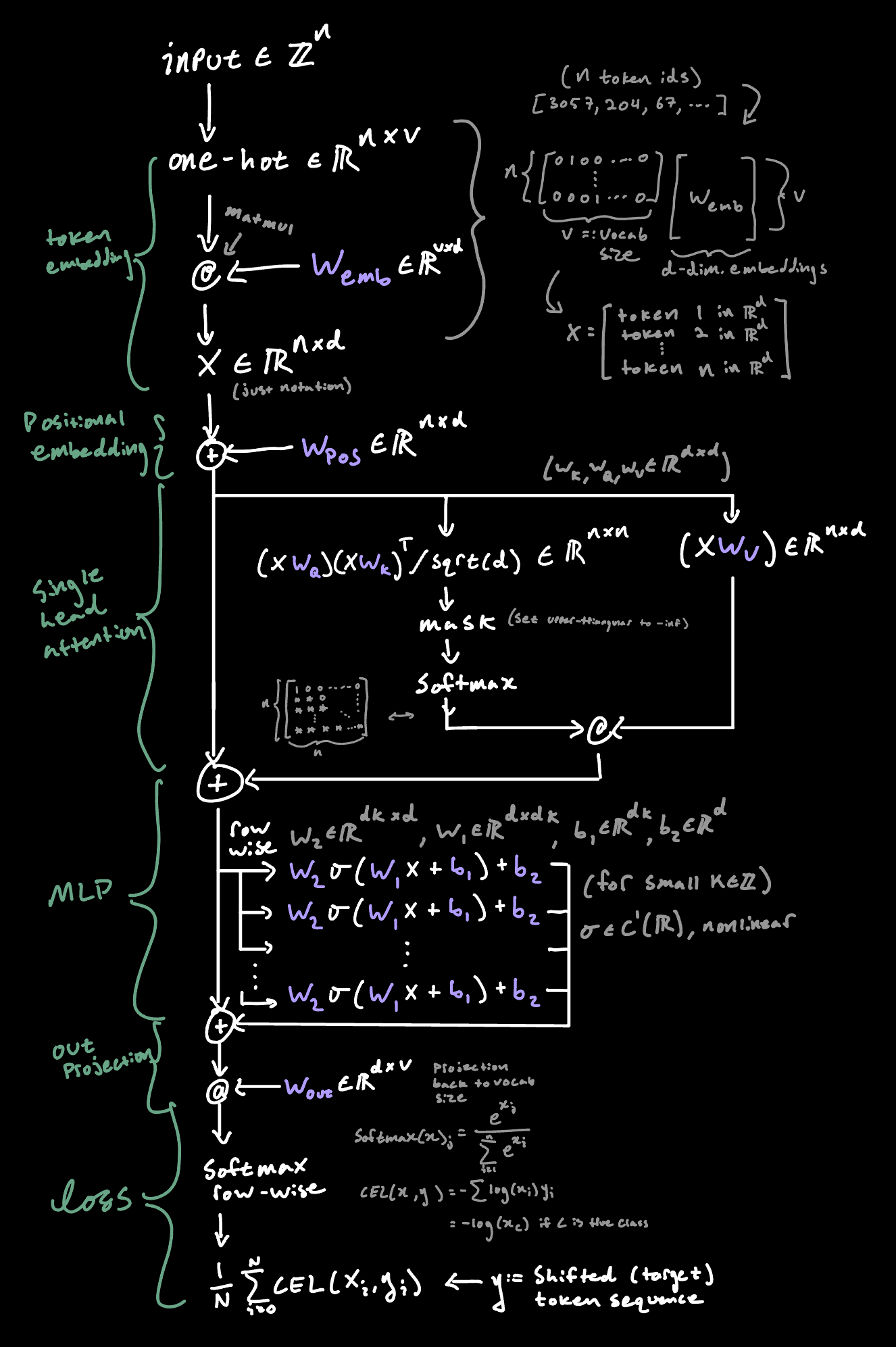
So now the question is: what can we do better?
naive multi head attention
First, let’s think about what the actual attention mechanism is doing. It’s taking in our input, ‘contextualizing’ token \(t_i\) with tokens \(t_{i-k}\) and then returning some ‘delta’ that’s added to our input.
Let’s also get in the habit now of calling the ‘input with stuff added to it as it flows through the network’ the ‘Residual Stream’.
So the attention mechanism is responsible for computing the actual attention mask (the \(n \times n\) shaped \(QK^T\) part), then using that to compute some function of our input (the \(V\) part) which gets added on to the residual stream.
The problem here is that the space where \(X\) is projected via \(W_V\) is responsible for encoding all the things you might want to push onto the residual stream. If we’re looking at a sequence that’s like “things I enjoy: apples, pie, ice cream”, then \(W_V\) is responsible not only for encoding “things following positive words like ‘enjoy’ should get pushed more positively” but also “things following ‘:’ should probably feel more list-y to the downstream MLP. And the attention mask is the same for all semantic information; it has to pay attention to the grammatical structure and the actual ‘vibes’ or meaning of the preceding text.
The fix seems pretty clear: just run a bunch of different attention mechanisms in parallel!
But then the question becomes: well our residual stream only takes things in \(R^{n \times d}\) so how do we actually wire this up?
One option is to just sum them, but then the output is just a fuzzy average of each head. What we really want is for the model to be able to ‘look at’ which head a given feature came from, and the feature index itself. This way the model can theoretically say “head 2 only tracks grammatical information so it shouldn’t push or pull on the sentiment dimension” (roughly speaking).
The shape that makes this work is:
\(\mathrm{MultiHead} = \mathrm{concat}(\mathrm{head}_1, \dots, \mathrm{head}_h)W_O\)
Where \(\mathrm{head}_i\) is the \(i^{th}\) attention ‘head’ and \(W_O \in \R^{hd \times d}\)
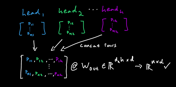
In code it looks like this:
# (n, d) x h -> concat -> (n, dh) @ (dh, d) -> (n, d)
class MultiHeadAttention(nn.Module):
    def __init__(self, n, d, h):
        super().__init__()
        self.heads = nn.ModuleList([Attention(n,d) for _ in range(h)])
        self.W_O = nn.Parameter(torch.randn(d * h, d) / math.sqrt(d))

    def forward(self, x: torch.Tensor):
        return torch.cat([h(x) for h in self.heads], dim=-1) @ self.W_O
And the results?
with these hyperparameters:
vocab_size = 2048
ctx_len = 32
batch_size = 4096
n_heads = 4
embedding_dim = 256
mlp_dh_coeff = 8
mlp_dh = embedding_dim * mlp_dh_coeff
mlp_depth = 2
Run on a 48mb dataset of high-quality gutenberg texts, the
single-head model finishes with a validation perplexity of
67.68, and the multi-head version finishes with a
validation perplexity of 66.48.
It’s not a massive difference, but it helps! Also note that i’m gpu poor so i’m running this on a small dataset with limited context. The results would likely be more striking on a larger set. Still an improvement!
The thing that’s most striking is the single head version shows an
attention entropy of 1.177 at the end of training. The
multi-head version has the following per-head attention entropies:
[0.69, 0.158, 1.011, 0.861]
This is really interesting! One of the heads is nearly one-hot, and the others are fairly well-balanced. Clearly the different heads are doing different things. What are they doing exactly? We could look at the activations (intermediate model states) and see what’s lighting up, and which head attends to which tokens, but I’m going to leave that as an exercise for the reader. I might add a section later that looks at this once I’m using better models and more sensible hyperparameters.
For now, we just care that we pushed the test loss down. Great. Next.
dimension-reduced multi-head attention
The next thing to do is simply to push the attention mechanisms to work in a lower dimensional space.
Currently if a single head takes \(P\) parameters then a multi-head setup will take \(hP\) params. The question is: can we save some space by working in a lower dimensional space? In theory, if we’re using \(h\) heads, then each head has to care about fewer feature directions, and can do its job with a lower-dimensional representation. This means we get a smaller model which is nice.
The only thing to change is the shape of the attention weight matrices and the out projection: Just have them downproject to some \(d_k << d\)
# in Attention
self.W_Q = nn.Parameter(torch.randn(d,d_k) / self.sqrt_d)
self.W_K = nn.Parameter(torch.randn(d,d_k) / self.sqrt_d)
self.W_V = nn.Parameter(torch.randn(d,d_k) / self.sqrt_d)

# in MultiHeadAttention
self.W_O = nn.Parameter(torch.randn(d_k * h, d) / math.sqrt(d_k * h))
Also we need to choose some value for \(d_k\). If you cheat and look at the
literature the way people do it is just set
d_k = embedding_dim // n_heads. This way the number of
parameters stays ~constant as we add more heads.
So does it work? Yes! We end up with a validation ppl of
65.11 which beats the full-rank multi-head attention and
uses fewer parameters! It’s a little unexpected that we actually
gain performance here. With such small models on such small
datasets, we should take this with a grain of salt. The point is we’re
not worse off doing this and we save a few parameters.
n-layer attention/mlp (transformers)
You already know what time it is. W’s in chat let’s stack some layers. I am not even going to bother really pedagogically motivating this. I mean come on. It’s so obvious. When we wanted more MLP performance we used a wider and deeper network. Since it’s not clear what a ‘wider’ multi-head attention setup looks like the only option is to go deeper.
Better yet, the change is trivial: we just do the
embedding/positional encoding, then pass that through a bunch of
multi-head attention/mlp blocks, then out with the W_out
projection and we’re done. Each ‘block’ is just adding a new delta
(recall, of shape \(\R^{n \times d}\))
to the residual stream.
class TransformerBlock(nn.Module):
    def __init__(self, n, d, h, d_k, mlp_dh, mlp_depth):
        super().__init__()

        self.attention = MultiHeadAttention(n,d,h,d_k)
        self.mlp = MLP(d, mlp_dh, mlp_depth)

    def forward(self, x: torch.Tensor):
        x = x + self.attention(x)
        return x + self.mlp(x)


class Transformer(nn.Module):
    def __init__(self, tokenizer, n, d, h, d_k, n_blocks, mlp_dh, mlp_depth):
        super().__init__()
        # ...
        self.W_pos = nn.Parameter(torch.randn(n, d))
        self.W_out = nn.Parameter(torch.randn(d, self.vocab_size) / math.sqrt(d))
        self.embedding = nn.Embedding(self.vocab_size, d)

        self.blocks = nn.Sequential(*[
            TransformerBlock(n, d, h, d_k, mlp_dh, mlp_depth)
            for _ in range(n_blocks)
        ])

    # x: (b, n) |-> (b, n, vocab_size)
    def forward(self, x: torch.Tensor):
        x = self.embedding(x) + self.W_pos  # (b,n) |-> (b,n,d)
        x = self.blocks(x)                  # (b,n,d) |-> (b,n,d)
        return x @ self.W_out               # (n d)(d vocab_size) = (n, vocab_size)
So how does it do? With 2 blocks, we get a final val perplexity of
55.74! Way better than the single block model. The training
dynamics look a little sketchy, the first block’s attention masks are
almost entirely one-hot by the end of training:
[0.036, 0.013, 0.006, 0.01] but that’s not a big deal if
the final val loss is down!
The generation quality is quite bad still, but it does look like we’re still marginally improving.
PROMPT:  ': in what circumstances then? must it not be in the most honourable? now such is death in war, because it is death in the'
OUTPUT:  'world, in which he has to do with that of a man who has been to the mind in his own nature, and as the predicate of a thing, and which is not so much as to think. It is a true cause. It is, that the whole in the United States are an objective reality, and is only in the mind (II. xiii.. and therefore (III. xi. not'
Now let’s try 4 blocks:
main | INFO | 2026-02-19 19:54:34 | starting training:
n_params=23.1M, n_batches=3548, batch_size=4096, context_length=33, tokens_per_batch=135.2K, total_tokens=1.4B
main | INFO | 2026-02-19 19:55:00 | {'batch': '100/3548', 'epoch': '1/3', 'tokens_seen': '13.5M', 'attn_entropy': {0: [nan, nan, nan, nan], 1: [nan, nan, nan, nan], 2: [nan, nan, nan, nan], 3: [nan, nan, nan, nan]}, 'batch_time_ms': 227.23, 'train_loss': nan, 'train_ppl': nan, 'val_loss': -inf, 'val_ppl': 0.0}
Shit.
RMSnorm
Well the attention masks are ‘blowing up’ again. Fortunately, we’ve seen this before. Recall the single-head attention post last time, when we tried doing attention without the \(\sqrt{d}\) scaling. What happened? The variance in the last dimension (ie per-row,per-position) was too high, and so one entry dominated the softmax, killed the gradient flow, and ruined our model. The fix was to normalize down to unit variance by dividing by the standard deviation.
Is the same thing happening here? Does the same fix work?
If we simply assume a mean of zero (it turns out that our residual stream does tend to center around zero), then the scaling factor would be:
\[\sqrt{\frac{1}{d}\sum_{i=1}^d x_i^2}\]
i.e. rescale by dividing by the standard deviation with an assumed mean of zero i.e.
transformer_block_input = residual_stream.pow(2).mean().sqrt()
Also observe (with some handwaving):
\[\mathbb{E}[||x||_2^2] = \mathbb{E}\left[\sum_{i=1}^d x_i^2\right] = \sum_{i=1}^d \mathbb{E}[x_i^2] = \sum_{i=1}^d 1 = d \implies \mathbb{E}[||x||_2] \approx \sqrt{d}\]
The right hand side is just there to illustrate the rough intuition that the scaling factor is roughly \(1\) (ie does little) if our input is already unit variance.
Hence our scaling factor here is something like \(\sqrt{d}/\sqrt{d} = 1\)
In other words, if the residual stream is already nice, we’re not doing anything. If the residual stream has a huge variance, we’re normalizing it.
There are two remaining issues with this potential fix.
First, if \(x\) is near zero, we’re going to encounter numerical instability. The fix is to add some \(\varepsilon \approx 0.000001\) inside the square root.
Second, we’re adding inductive bias here. It’s true that we do not want high variance in our residual stream, but also we’re scaling it in a very particular way. To let the model choose how to re-scale after normalization, we can add an elementwise multiplication by some learned parameter \(\gamma \in \R^d\).
We call this ‘rescaling’ RMSnorm (root mean square) and the final form is this: \[ \mathrm{RMSnorm}(x) = \gamma \odot \frac{x}{\sqrt{\varepsilon + \frac{1}{d}\sum_{j=1}^d x_j^2}} \]
The operation is broadcasted across the rows of \(x\). We apply it not to the main residual stream, but to the inputs of each attention and MLP block.
In code:
class RMSNorm(nn.Module):
    def __init__(self, d):
        super().__init__()
        self.gamma = nn.Parameter(torch.ones(d))

    def forward(self, x: torch.Tensor):
        rms = torch.sqrt(torch.mean(x ** 2, dim=-1, keepdim=True) + 1e-6)
        return self.gamma * (x / rms)

class TransformerBlock(nn.Module):
    def __init__(self, n, d, h, d_k, mlp_dh, mlp_depth):
        super().__init__()

        self.attention = MultiHeadAttention(n,d,h,d_k)
        self.mlp = MLP(d, mlp_dh, mlp_depth)
        self.rms1 = RMSNorm(d)
        self.rms2 = RMSNorm(d)

    def forward(self, x: torch.Tensor):
        x = x + self.attention(self.rms1(x))
        return x + self.mlp(self.rms2(x))
And the results are good! Running the network with this change gets
us a validation ppl of 48.99 on the same set we’ve been
using for a while now. In fact, this is the best we’ve managed to
do!
And at this point… we have the transformer! It’s worth noting that the version we’re running here was the version that we’ve pieced together over the course of the post. This means we’re doing some ‘non-standard’ things. To name a few: still using vanilla SGD, using 3 layers in the MLP blocks, using RMSnorm before the attention/mlp blocks instead of e.g. layer norm after, probably using some suboptimal hyperparameters, (fairly arbitrary hidden size in the mlp), etc…
The reason for these changes from the Attention Is All You Need version is because it seemed more pedagogically tractable/honest to go this route (using whatever seemed reasonable based on the logic for implementing it, rather than the empirical state of the art).
Finally, there are (at least) two more obvious problems with the network, so i’ll leave it as an exercise to the reader to guess what they are and what we’re going to do about it in the next post. Maybe you can diagnose them from the log of the last training run:
(note that g:=rms(gradient),
w:=rms(weights), u := lr * u/w; i.e. ‘how big
are the gradient/weight entries, on average, for this layer, and what
fraction of the weights get updated each step’)
sgd_transformer | INFO | 2026-03-01 14:45:41 | Sample generations (temperature = 0.0):
PROMPT:  'pleasure contrary to his Reason, the former feels but does not yield to it. Like again are the man of Imperfect'
OUTPUT:  'ly punish’d. Theirs are not to be found. Their figure is to be found. Theirs are not to be found. Theirs are not to be found. Theirs are not to be found. Their population is not to be found in the same way. The same is the same with which the same is the same, and the same is the same with the same, and the same is'

main | INFO | 2026-02-20 20:41:11 | {'batch': '3400/3548', 'epoch': '3/3', 'tokens_seen': '459.6M', 'attn_entropy': {0: [2.242, 2.243, 2.277, 1.515], 1: [0.855, 0.89, 1.004, 0.904], 2: [1.528, 1.332, 1.847, 1.545], 3: [1.516, 1.174, 1.976, 1.363]}, 'batch_time_ms': 294.81, 'train_loss': 3.311, 'train_ppl': 27.412, 'val_loss': 3.919, 'val_ppl': 50.369}
main | INFO | 2026-02-20 20:41:42 | gradient info:
    W_pos                               g=2.4e-04 w=9.9e-01 u=1.2e-05
    W_out                               g=7.0e-04 w=6.7e-02 u=5.2e-04
    embedding.weight                    g=3.1e-05 w=1.0e+00 u=1.6e-06
    blocks.0.attention.W_O              g=3.7e-04 w=5.2e-02 u=3.6e-04
    blocks.0.attention.heads.0.W_Q      g=5.5e-05 w=5.8e-02 u=4.8e-05
    blocks.0.attention.heads.0.W_K      g=5.4e-05 w=5.9e-02 u=4.6e-05
    blocks.0.attention.heads.0.W_V      g=3.3e-04 w=5.2e-02 u=3.2e-04
    blocks.0.attention.heads.1.W_Q      g=6.0e-05 w=6.1e-02 u=4.9e-05
    blocks.0.attention.heads.1.W_K      g=6.3e-05 w=6.2e-02 u=5.1e-05
    blocks.0.attention.heads.1.W_V      g=4.8e-04 w=5.3e-02 u=4.6e-04
    blocks.0.attention.heads.2.W_Q      g=6.0e-05 w=6.0e-02 u=5.0e-05
    blocks.0.attention.heads.2.W_K      g=6.2e-05 w=6.0e-02 u=5.2e-05
    blocks.0.attention.heads.2.W_V      g=4.2e-04 w=5.3e-02 u=3.9e-04
    blocks.0.attention.heads.3.W_Q      g=5.4e-05 w=5.9e-02 u=4.5e-05
    blocks.0.attention.heads.3.W_K      g=5.5e-05 w=5.9e-02 u=4.7e-05
    blocks.0.attention.heads.3.W_V      g=3.2e-04 w=5.2e-02 u=3.1e-04
    blocks.0.mlp.net.0.weight           g=3.2e-04 w=3.8e-02 u=4.3e-04
    blocks.0.mlp.net.0.bias             g=6.1e-04 w=3.9e-02 u=7.8e-04
    blocks.0.mlp.net.2.weight           g=2.1e-04 w=1.4e-02 u=7.8e-04
    blocks.0.mlp.net.2.bias             g=6.2e-04 w=1.3e-02 u=2.3e-03
    blocks.0.mlp.net.4.weight           g=6.5e-04 w=2.0e-02 u=1.7e-03
    blocks.0.mlp.net.4.bias             g=2.6e-03 w=1.8e-02 u=7.4e-03
    blocks.0.rms1.gamma                 g=4.2e-04 w=7.2e-01 u=2.9e-05
    blocks.0.rms2.gamma                 g=7.8e-04 w=1.1e+00 u=3.5e-05
    blocks.1.attention.W_O              g=8.5e-04 w=5.9e-02 u=7.2e-04
    blocks.1.attention.heads.0.W_Q      g=1.6e-04 w=6.3e-02 u=1.3e-04
    blocks.1.attention.heads.0.W_K      g=2.7e-04 w=6.2e-02 u=2.2e-04
    blocks.1.attention.heads.0.W_V      g=1.1e-03 w=6.0e-02 u=9.1e-04
    blocks.1.attention.heads.1.W_Q      g=1.9e-04 w=6.3e-02 u=1.5e-04
    blocks.1.attention.heads.1.W_K      g=2.8e-04 w=6.3e-02 u=2.3e-04
    blocks.1.attention.heads.1.W_V      g=1.0e-03 w=6.0e-02 u=8.4e-04
    blocks.1.attention.heads.2.W_Q      g=1.7e-04 w=6.3e-02 u=1.4e-04
    blocks.1.attention.heads.2.W_K      g=3.0e-04 w=6.3e-02 u=2.4e-04
    blocks.1.attention.heads.2.W_V      g=1.1e-03 w=6.0e-02 u=9.3e-04
    blocks.1.attention.heads.3.W_Q      g=1.6e-04 w=6.3e-02 u=1.3e-04
    blocks.1.attention.heads.3.W_K      g=2.6e-04 w=6.2e-02 u=2.1e-04
    blocks.1.attention.heads.3.W_V      g=9.4e-04 w=5.9e-02 u=7.9e-04
    blocks.1.mlp.net.0.weight           g=5.5e-04 w=4.2e-02 u=6.4e-04
    blocks.1.mlp.net.0.bias             g=8.8e-04 w=3.6e-02 u=1.2e-03
    blocks.1.mlp.net.2.weight           g=5.0e-04 w=1.6e-02 u=1.6e-03
    blocks.1.mlp.net.2.bias             g=1.2e-03 w=1.3e-02 u=4.5e-03
    blocks.1.mlp.net.4.weight           g=1.0e-03 w=2.8e-02 u=1.9e-03
    blocks.1.mlp.net.4.bias             g=4.0e-03 w=1.8e-02 u=1.1e-02
    blocks.1.rms1.gamma                 g=1.3e-03 w=9.2e-01 u=6.9e-05
    blocks.1.rms2.gamma                 g=8.6e-04 w=1.4e+00 u=3.1e-05
    blocks.2.attention.W_O              g=9.5e-04 w=5.7e-02 u=8.3e-04
    blocks.2.attention.heads.0.W_Q      g=2.1e-04 w=6.3e-02 u=1.7e-04
    blocks.2.attention.heads.0.W_K      g=2.8e-04 w=6.3e-02 u=2.2e-04
    blocks.2.attention.heads.0.W_V      g=1.3e-03 w=5.9e-02 u=1.1e-03
    blocks.2.attention.heads.1.W_Q      g=2.0e-04 w=6.3e-02 u=1.6e-04
    blocks.2.attention.heads.1.W_K      g=3.3e-04 w=6.3e-02 u=2.7e-04
    blocks.2.attention.heads.1.W_V      g=1.3e-03 w=5.9e-02 u=1.1e-03
    blocks.2.attention.heads.2.W_Q      g=2.3e-04 w=6.3e-02 u=1.8e-04
    blocks.2.attention.heads.2.W_K      g=3.9e-04 w=6.3e-02 u=3.1e-04
    blocks.2.attention.heads.2.W_V      g=1.2e-03 w=5.9e-02 u=1.1e-03
    blocks.2.attention.heads.3.W_Q      g=1.8e-04 w=6.2e-02 u=1.4e-04
    blocks.2.attention.heads.3.W_K      g=3.0e-04 w=6.2e-02 u=2.4e-04
    blocks.2.attention.heads.3.W_V      g=1.2e-03 w=5.9e-02 u=1.0e-03
    blocks.2.mlp.net.0.weight           g=5.0e-04 w=4.2e-02 u=5.9e-04
    blocks.2.mlp.net.0.bias             g=7.6e-04 w=3.5e-02 u=1.1e-03
    blocks.2.mlp.net.2.weight           g=4.4e-04 w=1.6e-02 u=1.4e-03
    blocks.2.mlp.net.2.bias             g=9.9e-04 w=1.3e-02 u=3.8e-03
    blocks.2.mlp.net.4.weight           g=8.7e-04 w=2.7e-02 u=1.6e-03
    blocks.2.mlp.net.4.bias             g=3.6e-03 w=1.6e-02 u=1.1e-02
    blocks.2.rms1.gamma                 g=1.6e-03 w=8.7e-01 u=9.3e-05
    blocks.2.rms2.gamma                 g=8.5e-04 w=1.4e+00 u=3.1e-05
    blocks.3.attention.W_O              g=9.6e-04 w=5.9e-02 u=8.2e-04
    blocks.3.attention.heads.0.W_Q      g=1.6e-04 w=6.3e-02 u=1.3e-04
    blocks.3.attention.heads.0.W_K      g=2.7e-04 w=6.3e-02 u=2.2e-04
    blocks.3.attention.heads.0.W_V      g=1.3e-03 w=6.1e-02 u=1.0e-03
    blocks.3.attention.heads.1.W_Q      g=1.6e-04 w=6.0e-02 u=1.3e-04
    blocks.3.attention.heads.1.W_K      g=3.3e-04 w=6.1e-02 u=2.8e-04
    blocks.3.attention.heads.1.W_V      g=1.6e-03 w=5.9e-02 u=1.3e-03
    blocks.3.attention.heads.2.W_Q      g=1.4e-04 w=6.3e-02 u=1.1e-04
    blocks.3.attention.heads.2.W_K      g=2.2e-04 w=6.3e-02 u=1.7e-04
    blocks.3.attention.heads.2.W_V      g=1.1e-03 w=6.0e-02 u=9.0e-04
    blocks.3.attention.heads.3.W_Q      g=2.0e-04 w=6.2e-02 u=1.6e-04
    blocks.3.attention.heads.3.W_K      g=3.2e-04 w=6.2e-02 u=2.6e-04
    blocks.3.attention.heads.3.W_V      g=1.3e-03 w=6.1e-02 u=1.1e-03
    blocks.3.mlp.net.0.weight           g=3.9e-04 w=4.4e-02 u=4.4e-04
    blocks.3.mlp.net.0.bias             g=4.9e-04 w=3.8e-02 u=6.5e-04
    blocks.3.mlp.net.2.weight           g=3.1e-04 w=1.6e-02 u=9.7e-04
    blocks.3.mlp.net.2.bias             g=5.1e-04 w=1.3e-02 u=2.0e-03
    blocks.3.mlp.net.4.weight           g=7.2e-04 w=2.9e-02 u=1.2e-03
    blocks.3.mlp.net.4.bias             g=1.3e-03 w=2.1e-02 u=3.2e-03
    blocks.3.rms1.gamma                 g=2.0e-03 w=8.7e-01 u=1.1e-04
    blocks.3.rms2.gamma                 g=9.3e-04 w=1.5e+00 u=3.2e-05main | INFO | 2026-02-20 20:41:sgd_transformer | INFO | 2026-03-01 14:48:08 | {'batch': '3500/3548', 'epoch': '3/3', 'tokens_seen': '473.1M', 'attn_entropy': {0: [2.315, 1.245, 1.714, 2.191], 1: [0.895, 0.996, 0.991, 1.095], 2: [1.432, 1.29, 1.312, 1.49], 3: [1.395, 1.998, 1.381, 1.497]}, 'batch_time_ms': 280.04, 'train_loss': 3.305, 'train_ppl': 27.253, 'val_loss': 3.901, 'val_ppl': 49.443}
sgd_transformer | INFO | 2026-03-01 14:48:42 | training finished w/ final val ppl=48.99362239152302
AdamW
Mar 1, 2026
The last post left off with a snippet of a training log, and we post the question “what’s wrong with our current setup?”
Look at the following two log chunks:
embedding.weight                    g=3.1e-05 w=1.0e+00 u=1.6e-06
blocks.0.attention.heads.0.W_Q      g=5.5e-05 w=5.8e-02 u=4.8e-05
blocks.0.attention.heads.0.W_K      g=5.4e-05 w=5.9e-02 u=4.6e-05
...

blocks.1.mlp.net.2.bias             g=1.2e-03 w=1.3e-02 u=4.5e-03
blocks.1.mlp.net.4.weight           g=1.0e-03 w=2.8e-02 u=1.9e-03
...
blocks.3.mlp.net.4.weight           g=7.2e-04 w=2.9e-02 u=1.2e-03
blocks.3.mlp.net.4.bias             g=1.3e-03 w=2.1e-02 u=3.2e-03
blocks.3.rms1.gamma                 g=2.0e-03 w=8.7e-01 u=1.1e-04
Sample generations (temperature = 0.0):
PROMPT: 'pleasure contrary to his Reason, the former feels but does not yield to it. Like again are the man of Imperfect'
OUTPUT: 'ly punish’d. Theirs are not to be found. Their figure is to be found. Theirs are not to be found. Theirs are not to be found. Theirs are not to be found. Their population is not to be found in the same way. The same is the same with which the same is the same, and the same is the same with the same, and the same is'fixing sgd: Adam
The first issue is that gradient norms vary by orders of magnitude across parameters. Gradients to our first attention layer are two OOMs smaller than the gradients to the first MLP.
Is this a problem? Well, stochastic gradient descent assigns gradient magnitudes based on the immediate loss landscape, not based on the distance to the optimum. So a smaller gradient doesn’t mean “we’re done” it literally just means “the local loss landscape around this parameter has less curvature”. So yeah, it could definitely be a problem.
Think about it- the update applied to each parameter is some constant fraction of the actual computed gradient. Recall the sgd formulation: \(\theta_t = \theta_{t-1} - \eta \nabla_\theta f(x,\theta_{t-1})\)
Imagine the optimal value of \(\theta\) sits at the bottom of a very steep hill. Then the gradient magnitudes are going to remain large, and the actual computed \(\theta\) is going to bounce around wildly, despite being “close” to the optimum in the context of the overall loss landscape.
On the other hand, if \(\theta\) is “far away” from the optimum, but the local loss topography is “shallow”, (ie the gradient magnitude is small), then it’s going to take forever for \(\theta\) to approach the optimum.
So currently we take steps proportional to the curvature of the local loss landscape. But it looks like what we want to do is take steps proportional to how far away from the optimum we are. And from that last example, we already have some intuition for how we might go about doing this:
In pseudocode, we’d write something like:
def get_gradient_scale(gradient_history):
    if are_generally_pointing_in_the_same_direction_for_a_while(gradient_history):
        return BIG_STEPSIZE   # high confidence we know where to go, can speed up
    else:
        return SMALL_STEPSIZE # gradients change wildly, uncertain or close to optimum
We just have to figure out how to formalize this. The first question is like … what is BIG_STEPSIZE and what is SMALL_STEPSIZE?
The nice thing about vanilla SGD is that we learn this from the function itself. It’s a method that works (subject to ‘oops, stuck in local minima’) over the massive class of real-valued differentiable functions.
That is, it works for functions like this:
\(f(x,y) = (x - 0.01)^2 + (y - 0.02)^2\) (optimum at small values)
and for functions like this:
\(f(x,y) = (x - 100)^2 + (y - 200)^2\) (optimum at large values)
The gradient at distance \(d\) from optimum is \(2d\), so it scales naturally. SGD with lr=0.1 works for both if you init reasonably.
But we don’t care about general functions here! We’re training a very particular class of neural network. And we’ve empirically observed in the training logs that all of our parameters are near the \(10^{-2}\) range.
So why not simply hardcode some reasonable base stepsize \(\alpha := 0.001\)?
Then for each (scalar) parameter, the update rule is just:
\[\theta_t = \theta_{t-1} - \alpha \cdot \mathrm{scale}(\nabla_1,\nabla_2, \dots, \nabla_{t-1})\]
Where \(\mathrm{scale}\) is some function of the gradient history, where:
\(\mathrm{scale} \approx 1\) when we’re taking ‘confident’ steps towards \(\infty\),
\(\mathrm{scale} \approx -1\) when we’re taking ‘confident’ steps towards \(-\infty\),
and \(\mathrm{scale} \approx 0\) when we’re taking ‘uncertain’ steps in either direction.
Admittedly this notation may be somewhat confusing. Here’s a sketch:
noise to signal ratio
The big question is just like … how do we mathematically express this magic \(\mathrm{scale}\) term as a function of the gradient history?
The first thing to do is figure out a way to determine how much directional noise we’re experiencing. A simple approach would just be to take the moving average. Entries in the gradient history which are additive inverses of one another cancel themselves out and push the number closer to zero, which is a good starting point in our search for a suitable expression.
Let \(g_t\) be the scalar gradient value of some entry in a weight matrix at step \(t\), and \(\mathrm{EMA}\) be the exponential moving average (exponential is easier to compute and more stable than a simple sliding-window moving average)
then: \[\mathrm{scale} = \mathrm{EMA}(g_t, g_{t-1}, \dots, g_1)\]
From there, we can normalize to the range \([-1,1]\) by dividing and taking care of the signs:
\[\mathrm{scale} = \frac{\mathrm{EMA}(g_t, g_{t-1}, \dots, g_1)} {\sqrt{\mathrm{EMA}(g_t^2, g_{t-1}^2, \dots, g_1^2)}}\]
Let’s pause. If the gradient history (recall we’re looking at one
entry in a vector so these are scalars) looks like:
[1,-1,1,-1,...], then the EMA on the top is near
0 (with many entries, small EMA \(\beta\) parameter), and 1 on
the bottom. If the gradient history is [1,1,1,1,...], the
numerator is 1 and the denominator is 1.
Good.
Let’s formalize it a bit and see if anything sticks out:
Let \(\alpha, \beta \in \R\). Set \(m_0, v_0 = 0\).
Loop over \(t\) until satisfied: \[ \begin{align} g_t &\leftarrow \nabla_\theta f_t(\theta_{t-1})\\ m_t &\leftarrow \beta \cdot m_{t-1} + (1-\beta) \cdot g_t\\ v_t &\leftarrow \beta \cdot v_{t-1} + (1-\beta) \cdot g_t^2\\ \theta_t &\leftarrow \theta_{t-1} - \alpha \cdot m_t / (\sqrt{v_t} + \epsilon)\\ \end{align} \]
Note what we’re doing. We’re computing the first moment (mean) on the top and the second moment (variance) on the bottom. We’re also computing moving averages, so these moments will be biased towards zero at the start. We can correct for this (don’t worry too much about this part):
\[ \begin{align} g_t &\leftarrow \nabla_\theta f_t(\theta_{t-1})\\ m_t &\leftarrow \beta \cdot m_{t-1} + (1-\beta) \cdot g_t\\ v_t &\leftarrow \beta \cdot v_{t-1} + (1-\beta) \cdot g_t^2\\ \hat{m_t} &\leftarrow m_t / (1 - \beta^t)\\ \hat{v_t} &\leftarrow v_t / (1 - \beta^t)\\ \theta_t &\leftarrow \theta_{t-1} - \alpha \cdot \hat{m_t} / (\sqrt{\hat{v_t}} + \epsilon)\\ \end{align} \]
But wait - why use the same \(\beta\) for both \(m\) and \(v\)? They’re doing different jobs.
\(m\) tracks direction - “where are we heading right now?” This should adapt relatively quickly. If the loss landscape changes, we want to notice within like ~10 steps.
\(v\) tracks scale - “what’s the typical magnitude of gradients for this parameter?” This should be stable. If the denominator \(\sqrt{v}\) fluctuates a lot, our effective learning rate becomes erratic. We want this to change slowly over training.
So we use a lower \(\beta_1 = 0.9\) for momentum (effective window ~10 steps, more responsive) and a higher \(\beta_2 = 0.999\) for the scale estimate (effective window ~1000 steps, very stable).
Set \(\beta_1 = 0.9\), \(\beta_2 = 0.999\) and do:
\[ \begin{align} g_t &\leftarrow \nabla_\theta f_t(\theta_{t-1})\\ m_t &\leftarrow \beta_1 \cdot m_{t-1} + (1-\beta_1) \cdot g_t\\ v_t &\leftarrow \beta_2 \cdot v_{t-1} + (1-\beta_2) \cdot g_t^2\\ \hat{m_t} &\leftarrow m_t / (1 - \beta_1^t)\\ \hat{v_t} &\leftarrow v_t / (1 - \beta_2^t)\\ \theta_t &\leftarrow \theta_{t-1} - \alpha \cdot \hat{m_t} / (\sqrt{\hat{v_t}} + \epsilon)\\ \end{align} \]
And that’s the Adam optimizer! Note that these moving averages are cheap to compute, and give us full per-parameter adaptive learning rates.
Let’s try it out! We’ll start with the same learning rate we used for SGD. And conveniently in pytorch this is a one line change.
optimizer = optim.Adam(params = model.parameters(), lr = 0.05)empirical results
Let’s start training!
adam | INFO | 2026-03-01 16:58:54 | starting training:
n_params=23.1M, n_batches=3548, batch_size=4096, context_length=33, tokens_per_batch=135.2K, total_tokens=1.4B
Traceback (most recent call last):
  File "/home/anon/projects/ml2/ml9/adam.py", line 509, in <module>
    main()
  File "/home/anon/projects/ml2/ml9/adam.py", line 506, in main
    train(training_state, logger)
  File "/home/anon/projects/ml2/ml9/adam.py", line 439, in train
    state.log_batch(batch_no + 1, logger)
  File "/home/anon/projects/ml2/ml9/adam.py", line 330, in log_batch
    'train_ppl': round(math.exp(self.train_loss), 3),
                       ^^^^^^^^^^^^^^^^^^^^^^^^^
OverflowError: math range error
Hmmm. Yeah that’s not going to work. Let’s try the default
lr=1e-3.